Regression is predictive modeling. It is a statistical method used in finance, investment, and other disciplines that attempts to determine the strength and character of the relationship between one dependent variable (usually denoted by Y) and a series of other variables (known as independent variables).
Regression helps investment and financial managers value assets and understand the relationships between variables, such as commodity prices and the stocks of businesses dealing in those commodities.

Notes:

The Reader (Dataset) should be connected to the algorithm.
Missing values should not be present in any rows or columns of the reader. Use the Descriptive Statistics algorithm to check whether there are any missing values. Refer to Descriptive Statistics
If missing values are present, impute them using the Missing Value Imputation algorithm on the dataset. It is under Model Studio in Data Preparation.
The dependent or output variable (y) must be a continuous data type. It should be a numerical variable.

Linear Regression

Description	Linear regression is a statistical and ML method to establish a linear relationship between the input variables (x) and a single output variable (y). The value of y can be calculated from a linear combination of variables x.
Why to use	To perform the Predictive Modeling for the dependent variable.
When to use	When you want to predict a value depending upon single or multiple independent variables.	When not to use	On textual data.
Prerequisites	There should not be any missing values in the data. The output variable (y) must be a continuous data type. Linearity: The relationship between x and y is linear. Homoscedasticity: Residual variance is the same for any value of x. Independence: There is no correlation in the independent variables. Normality: Residuals must be normally distributed.
Input	A single numeric Dependent variable A set of Independent variables, a combination of numeric and categorical variables	Output	Predicted value.
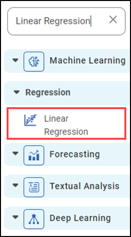
Statistical Methods used	Regression Mean ANOVA R square Adjusted R square Residual Coefficient Significance level (alpha) Durbin Watson – Auto Correlation Factor Variance Inflation Factor p value W Statistic	Limitations	It cannot be used on textual data. It is sensitive to Outliers. It is limited to linear relationships.

Linear Regression is located under Machine Learning ( ) in Regression, in the task pane on the left. Use the drag-and-drop method to use the algorithm in the canvas. Click the algorithm to view and select different properties for analysis. Refer to Properties of Linear Regression.

The equation for linear regression is, y=mx+c

y is the dependent variable (output)
m is the slope or weight
x is the independent variable (input)
c is the constant or intercept

The output variable is the dependent variable or scalar response, while the input variables are independent or explanatory. The output variable (y) must be a continuous data type.
There are two types of linear regression, simple and multiple. In simple linear regression, there is only one input variable (x), while in multiple linear regression, there are multiple input variables (x1,x2,x3,x4). As input variables increase, slopes or weights will also increase.
Linear regression aims to determine which predictors are significant in predicting the output variable, their efficiency in predicting the output variable, and how they impact the output variable.

Properties of Linear Regression

The available properties of Linear Regression are shown in the figure below.

The table below describes the different fields present in the properties of Linear Regression.

Field		Description	Remark
Task Name		It displays the name of the selected task.	You can click the text field to edit or modify the task's name as required.
Dependent Variable		It allows you to select the variable from the drop-down list for which we need to predict the values of the dependent variable y.	Only one data field can be selected. Numerical data fields of only those data fields that are selected for the reader are visible.
Independent Variables		It allows you to select the experimental or predictor variable(s) x.	Multiple data fields can be selected. Numerical data fields of only those data fields that are selected for the reader are visible. Set encoding method for categorical variables.
Stepwise Regression		It allows the user to select methods of stepwise regression.	It contains the values like Forward Selection, Backward Elimination, and Bidirectional Selection. By default, the Forward selection method is selected.
Advanced	Variance Inflation Factor	It allows you to detect multicollinearity in regression analysis.	You can either select True or False. Selecting True calculates the Variance Inflation Factor and displays it in result pane. Selecting False will disable the VIF function. It will remove the Variance Inflation Factor table from the result pane. By default, it is selected as False.
Advanced	Fit Intercept	It allows you to select whether you want to calculate the value of constant (c) for your model.	You can either select True or False. Selecting True calculates the value of the constant. By default, it is selected as True.
Dimensionality Reduction		It allows you to select the dimensionality reduction option. There are two parameters available None Principal Component Analysis (PCA)	If you select PCA, another field is created for inserting the variance value. Select a suitable value of variance.
Add Result as a variable		It allows you to select whether the result of the algorithm is to be added as a variable.	For more details, refer to Adding Result as a Variable.
Node Configuration		It allows you to select the instance of the AWS server to provide control over the execution of a task in a workbook or workflow.	For more details, refer to Worker Node Configuration
Hyper Parameter Optimization		It allows you to select parameters for optimization.	For more details, refer to Hyper parameter Optimization

Stepwise Regression Methods

You can choose either of the following iterative regression methods in Machine Learning.

Forward Selection
- It starts with no variable in the model.
- The system adds one variable in the model and checks whether the model is statistically significant.
- If the model is statistically significant then the variable is added to the model.
- The above steps are repeated till the system gets optimal results.
Backward Elimination
- It starts with a set of independent variables.
- The system removes one variable from the model.
- Then checks whether the model is statistically significant. If the model is not statistically significant then the variable is removed from the model.
- The above steps are repeated till the system gets optimal results.
Bidirectional Selection
- It is a combination of the Forward selection and Backward elimination methods.
- It adds and removes the independent variable combinations. Checks if the model is statistically significant.
- Repeat the steps till it gets all the independent variables between the significant level.

Example of Linear Regression

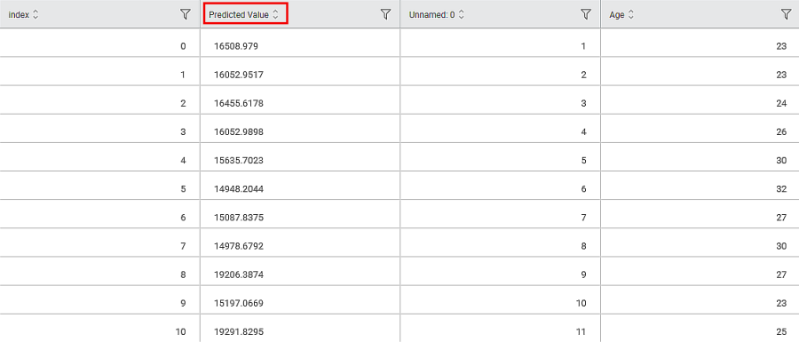
The Linear Regression is applied to a Used car dataset in the example below. Price is a dependent variable, and Age, Kilometer (KM), HorsePower(HP), and Cubic Capacity (CC) are independent variables. The data tab contains the Predicted Value for a dependent variable based on Independent variables as follows:

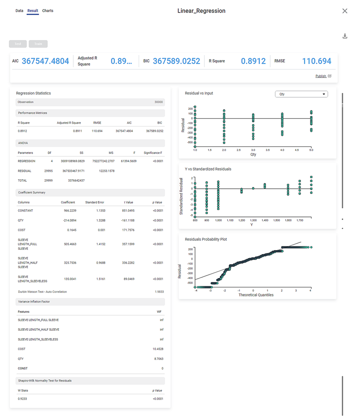
The Result page of Linear Regression is shown below.

The result page is segregated into the following sections.

Key Performance Indicator (KPI)
Regression Statistics
Graphical representation

Section 1: Key Performance Indicator (KPI)
The figure below displays various KPIs calculated in Linear Regression.

The table below describes multiple (KPIs) on the result page.

Performance Metric	Description	Remark
AIC (Akaike Information Criterion)	AIC is an estimator of errors in predicted values and signifies the quality of the model for a given dataset.	A model with the least AIC is preferred.
Adjusted R Square	It is an improvement of R Square. It adjusts for the increasing predictors and only shows improvement if there is a real improvement.	Adjusted R Square is always lower than R Square. In this example, there is not much difference between Adjusted R Square and R Square. In other words, you have considered most of the predictors in this regression.
BIC (Bayesian Information Criterion)	BIC is a criterion for model selection amongst a finite set of models.	A model with the least BIC is preferred.
R Square	It is the statistical measure that determines the proportion of variance in the dependent variable that is explained by the independent variables.	Value is always between 0 and 1. In this example, the regression model is a good fit with observed values.
RMSE (Root Mean Squared Error)	It is the square root of the averaged squared difference between the actual and predicted values.	It is the most commonly used metric to evaluate the model's accuracy. The model with lower RMSE is preferred.

Section 2: Regression Statistics
Regression Statistics consists of ANOVA, Performance Metrices, Coefficient Summary, Durbin Watson Test - Auto Correlation, Variance Inflation Factor, and Shapiro-Wilk Normality Test for Residuals for each of the selected independent (predictor) variables.
The Observation displays the total number of rows considered in Linear Regression.

The Performance Metrices consist of all KPI Details.
The ANOVA test calculates the difference in independent variable means. It helps you distinguish the difference in the behavior of the independent variable. To know more about ANOVA, click here.
You see values like Degrees of Freedom (DF), Sum of Squares (SS), Mean Sum of Squares (MS), F statistic of ANOVA, and Significance F.
DF represents The number of independent values that can differ freely within the constraints imposed on them.
SS is the sum of the square of the variations. Variation is the difference (or spread) of each value from the mean.
MS is the value obtained by dividing the Sum of Squares by Degrees of Freedom
F statistic of ANOVA indicates whether the regression model provides a better fit than a model without independent variables.

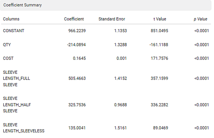
The Coefficient Summary displays the coefficient correlation between a dependent variable and each independent variable. If the coefficient of correlation is less than zero then there is a negative correlation between the dependent and an independent variable. In this example, there is a negative correlation between Age and KM.
It also calculates the p value based on the t statistic. The null hypothesis is rejected if the p value is less than level of significance (alpha). In the given example, the p value is less than level of significance (alpha).

The Durbin Watson Test determines autocorrelation between the residuals. If the test value is less than 2 then there is a positive correlation in the sample.
To find out more details about the Durbin Watson test, Click here

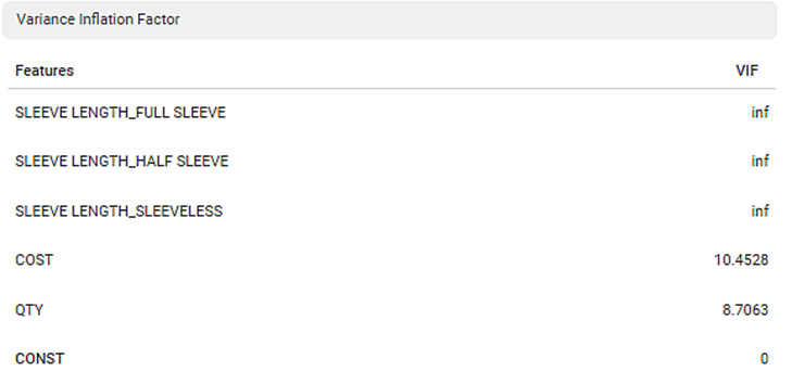
The Variance Inflation Factor is used to detect multicollinearity in regression analysis. VIF is calculated by selecting one predictor and regressing it against all other predictors in the model.
The value of VIF is equal to or greater than 1. If VIF = 1, the predictors are not correlated. If VIF is between 1 and 5, they are moderately correlated. For any value greater than 5, the predictors are heavily correlated. The higher the value of VIF, the lower the reliability of the regression results, and ultimately the model.

The Shapiro-Wilk Normality Test for Residuals test checks if the input data comes from a normal distribution. If the p value is less than 0.05 then reject the null hypothesis. In the given example, the p value is less than 0.05; hence the null hypothesis is rejected. To find out more details about Shapiro-Wilk Normality Test, Click here

Section 3: Graphical representation

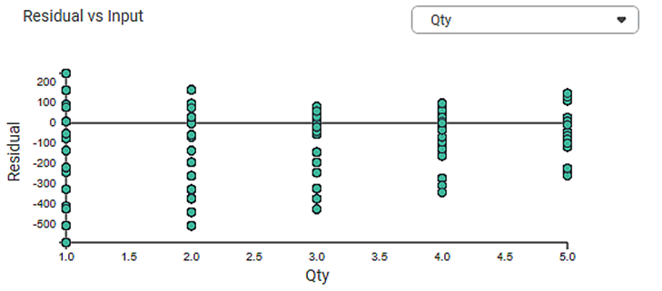
1. Residual vs. Input graph:

If this graph creates a pattern, then the sample is improper.
The graph is plotted with the Independent variable on the x-axis and Residual points on the y-axis.
On the right side, there is an independent variable dropdown. In this example, independent variables like Age, KM, HP, and CC appear in the dropdown.
The input variable is the same as in the dropdown. In the figure below, the input variable is Age, the same as in the dropdown.
If this graph follows a pattern then the data is not normally distributed.

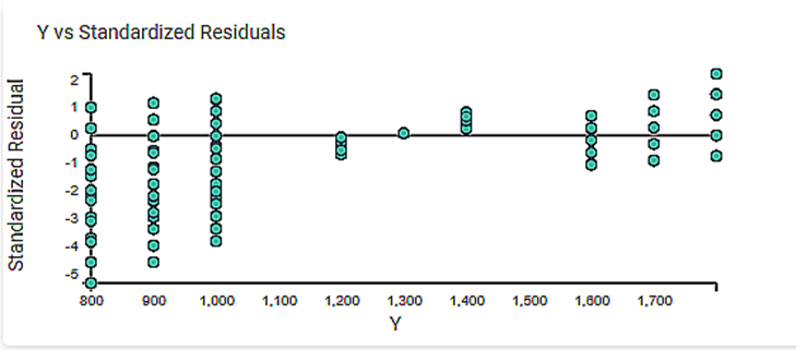
2. The Y vs. Standardized Residuals graph plots the dependent variable, Price, on the x-axis and the Standardized Residual on the y-axis.

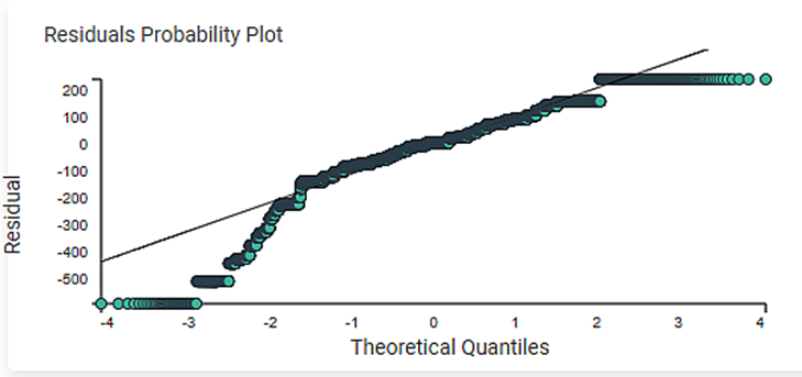
3. The Residuals Probability Plots the Independent variable on the x-axis and standardized Residuals on the y-axis. It helps to identify whether the error terms are normally distributed.

4. The Best Features displays the order of the Independent variable that provides the best result of R². You have performed linear regression with the backward compatibility method in this example. The best sequence of the independent variable is Age, KM, HP, and CC. This order is based on the adjusted R².

Table of Contents