Accuracy

Accuracy (of classification) of a predictive model is the ratio of the total number of correct predictions made by the model to the total predictions made. Thus,
Accuracy = (TP + TN) / (TP + TN + FP + FN)
Where,
TP, TN, FP, and FN indicate True Positives, True Negatives, False Positives, and False Negatives respectively.
Multiplying this ratio by 100 converts it into a percentage. Model classifiers have a 100% accuracy, while in reality, it is not possible.
Many times, classification accuracy can be misleading. Hence it is desirable to select a model with a slightly lower accuracy because it has a higher predictive power in the classification problem.
See also,

• Confusion Matrix
• False Positive
• True Negative
• True Positive
• False Negative

Adaboost

Adaboost, a short form of Adaptive Boosting, is one of the pioneering ML meta-algorithm, which is used for binary classification. It combines multiple weak classifiers into a weighted sum and gives the final output of a single strong boosted classifier. Generally, it is used with short decision trees.
Adaboost chooses a training set based on the accuracy of the previous training. Thus, it retains an algorithm iteratively. Also, the weight and age of each trained classifier at any iteration depends on the level of accuracy achieved.
Adaboost training process selects only those features which improve the predictive power of the model. Thus, irrelevant features are not computed, dimensionality is reduced, and execution time is improved.
Adaboost is sensitive to noisy data and outliers. It can be less susceptible to the over-fitting problem as compared to other learning algorithms.
See also,

• rubiML
• Machine Learning Algorithms

Akaike Information Criterion (AIC)

Akaike Information Criterion (AIC) is a technique to compare different models based on a given outcome. It is based on in-sample fitting and measures how well a model estimates future values. Technique based on in-sample fit to estimate the likelihood of a model to predict/estimate the future values.

AIC= –[2×ln(L)]+ [2×k]

Where,
L = value of the likelihood
k = number of estimated parameters Statistical models are used to represent processes that generate in-sample data. No model is 100% accurate and will more or less lead to loss of some information. AIC determines this relative loss of information caused by various models that are being compared. Lower the information lost, higher is the model quality. The best model is the one that has minimum AIC among the given models. Thus, AIC is a criterion for model selection. It also strikes a balance between the overfitting and underfitting of a model.
See also,
Bayesian Information Criterion (BIC)

Analysis of Variance (ANOVA)

Analysis of Variance (ANOVA) is a statistical technique that measures the difference between the means of two or more groups in a sample. It gives similar results to the t-test when used for two groups. However, it is predominantly used when three or more groups are to be compared. ANOVA is one of the methods to determine the significance of experimental results.
There are two types of ANOVA tests depending upon the number of independent variables – one-way and two-way. In the one-way test, there is one independent variable with two groups/levels. In the two-way test, there are two independent variables along with the possibility of multiple groups/levels. The two-way test can be performed with or without replication.
The computations of the ANOVA test statistic are arranged in an ANOVA table given below. It contains the values corresponding to Sum of Squares (SS), degrees of freedom (df), Mean Square (MS), and the F-value.

Table: ANOVA table

Where,
SSB = sum of squares between samples
SSW = sum of squares within samples
MSB = mean square between samples
MSW = mean square within samples
n = total sample size (sum of each of the sample sizes)
k = total number of treatments or observations (number of independent samples)
See also,

• Degree of Freedom (df)
• F-test of significance
• Sum of Squares (SS)
• Mean Square (MS)

Apriori

Apriori algorithm is a classic algorithm which is useful in mining frequent item-sets and relevant association rules. It is usually applied on a database that has a large number of recorded transactions like items purchased by customers at a supermarket.
The three important components of the apriori algorithm are support, confidence, and lift.
See also,
rubiML

Bayesian Information Criterion (BIC)

Bayesian Information Criterion (BIC), or Schwarz Information Criterion (abbreviated as SIC, SBC, or SBIC), is similar to Akaike Information Criterion (AIC) and is used as a method of model selection from a finite set of models.

Criteria for model selection that measures the trade-off between model fit and complexity of the model

BIC= –[2×ln(L)]+[2×ln(N)(k)]

Where,

L = value of the likelihood

N = number of recorded measurements

k = number of estimated parameters

Similar to the case of AIC, a model with lower BIC is usually preferred. BIC penalizes the complexity of a model. It adds a larger penalty term for the number of parameters in the model (compared to AIC), to overcome the problem of overfitting.

See also,

Akaike Information Criterion (AIC)

Binary Data

Binary data is a type of categorical data in which each unit or data point can take only two values.
For example, 0 and 1, True or False, Yes or No, and so on.

Binomial Logistic Regression

Binomial logistic regression, or simply logistic regression, uses the cumulative logistic distribution for making predictions. It is a prediction technique used to describe data and to explain the relationship between one dependent binary variable and one or more independent variables.
It predicts the probability that an observation falls into one of the two categories of a dichotomous (or binary) dependent variable based on one or more (categorical or continuous) independent variables.
For example, let study performance be a dependent variable measured on a dichotomous (binary) scale - pass or fail. Let revision time, test anxiety, and class attendance be the corresponding independent variables. Then binomial logistic regression can be employed to study the effect of the three independent variables on study performance.
See also,

• Regression
• Ridge Regression
• Lasso Regression
• Linear Regression
• Multinomial Logistic Regression

Box Plot

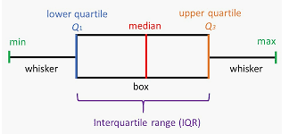
A box plot, or a box and whisker plot, is a graphical representation of the distribution of numerical data using its five values. These values are the minimum value, the first quartile, the median, the third quartile, and the maximum value.
It contains a box drawn between the two quartiles and two linear extensions (whiskers) on two sides to show the variation outside the lower and the upper quartile.
A typical box plot is shown below.

Figure: Box plot

Box plot is useful in descriptive data analysis to summarize data on an interval scale, show the distribution and concentration of data, the shape of the distribution, the central value, and the variability of the distribution.
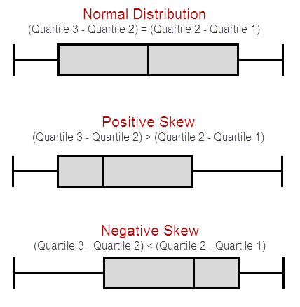
Box plots show whether a statistical dataset is normally distributed or skewed.

• If the dataset is symmetrically (normally) distributed, the median lies in the middle of the box and the whiskers are about the same length on both the sides.
• If the dataset is positively (or right) skewed, the median lies closer to the lower end of the box and whisker on that end is shorter.
• If the dataset is negatively (or left) skewed, the median lies closer to the upper end of the box and whisker on that end is shorter.

Figure: Normal and Skewed Distribution

See also,

• Outlier Detection
• Descriptive Statistics

Chi-square Test

The chi-square test is a statistical test used for testing relationships between categorical variables (not the numerical or continuous data) under a null hypothesis.
The null hypothesis of the Chi-square test states that no relationship exists between the categorical variables in the population, that is, they are independent. Whenever the observations don't fit the null hypothesis, the two variables are most likely to be dependent, and the null hypothesis is proved to be false.
The Chi-square test is a non-parametric statistic, also called a distribution-free test. Non-parametric tets should be used when any one of the following conditions pertains to the data: The level of measurement of all the variables is either nominal or ordinal.

Coefficient of correlation (R or r)

The coefficient of correlation is used in statistics to measure how strongly two variables are related to each other. Although there are many correlation coefficients, the most commonly used is Pearson's r.
The value of Pearson's r lies between -1 and 1. It is not affected by the shift of origin and the change of scale.
Negative value of r indicates an inverse relationship between the variables while a positive value of r indicates a direct relationship between them.
The Karl Pearson's correlation coefficient quantifies the strength of the linear relationship between two variables measured on an interval or a ratio scale.

Table: Values of r and their Interpretation

See also,
Coefficient of determination (R2)

Coefficient of determination (R²)

The coefficient of determination (R²) is the square of Pearson's R and is a measurement of the variance of one variable because of its relationship with another related factor.
Coefficient of determination is often called as proportion of variation, explained by the regressor x (independent variable).
This correlation between the two variables is also known as the goodness of fit and its values lie between 0 and 1.
The value R² = 1 indicates a perfect fit and model is highly reliable for forecasts in the future. It implies that most of the variability in the dependent variable y is explained by the regression model.
The value R² = 0 indicates that the model completely fails to model the data.
Some misconceptions about R²:

• It does not measure the magnitude of the slope of the regression line.
• It does not measure the appropriateness of the linear model.
• Large value of R² does not necessarily imply that the regression model will be an accurate predictor.

See also,
Coefficient of correlation (R or r)

Confusion Matrix

Confusion matrix (also called the error matrix) is a summary of the results of the predictions on a classification problem. It is used to calculate the performance of a classifier on a set of testing data where the true values are already known.
A confusion matrix helps us to visualize the performance of a classification algorithm.

Figure: Confusion Matrix

Source: https://www.saedsayad.com/model_evaluation_c.htm
See also,

• False Positive
• True Negative
• True Positive
• False Negative

Correlation

Correlation is a statistical technique that shows whether a pair of variables is related and, if yes, how strongly it is related.
Although the correlation may not be ideal, it gives a measure of the variation in one variable with the variation in another variable.

Correlation Matrix

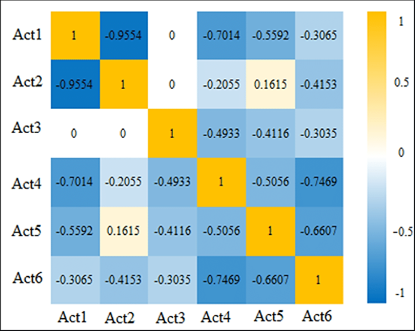
A correlation matrix is a table showing correlation coefficients between variables. While drawing a correlation matrix, we consider the choice of correlation statistic, coding of the variables, treatment of missing data, and the presentation of the matrix.
The correlation matrix summarizes data and is used as a precursor to, and a diagnostic tool for, advanced analysis.
A typical correlation matrix is shaped as a square where the same variables are shown in rows and columns.

Figure: Typical correlation matrix

Data Classification

Data classification is the process of tagging and organizing data according to relevant categories. This makes the data secure and searchable, easy to locate, and retrieve when needed.
Data classification can be content-based, context-based, or user-based.
See also,

• Decision Tree
• Gradient Boosting
• Naive Bayes
• Random Forest

Data Clustering

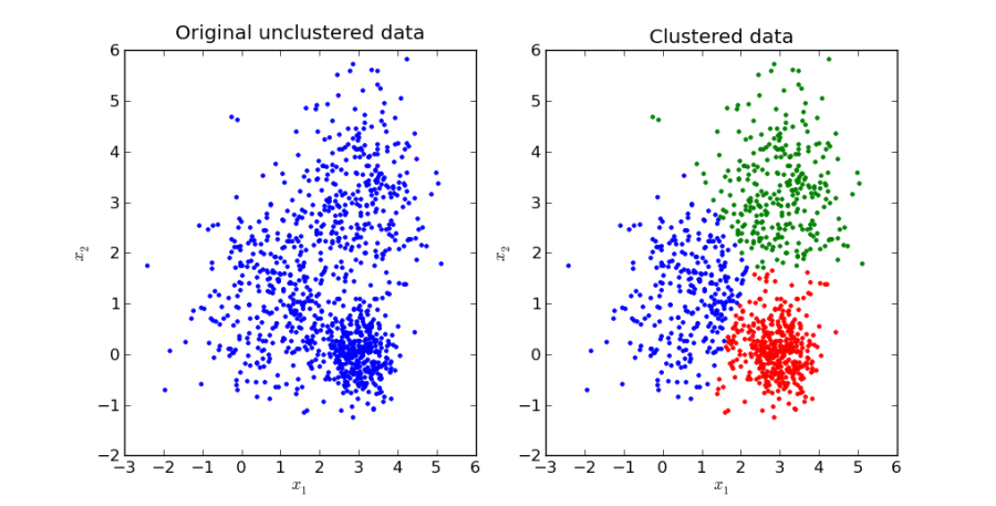
Data clustering (or cluster analysis) is a method of dividing the data points into several groups called clusters. All data points within a cluster are mutually similar as compared to data points belonging to different clusters. Thus, clusters are groups segregated based on identical traits.
Clustering can be hard or soft. In hard clustering, a data point either belongs to a cluster completely or does not belong to a cluster at all. In soft clustering, the probability of a data point belonging to a cluster is determined.

Figure: Clustering of data from unclustered data

Data Exploration

Data exploration (or exploratory data analysis) is a method by virtue of which we understand, summarize, and analyse the contents of a dataset to investigate a specific question or to prepare for advanced modelling. Data exploration is an initial step of data analysis, which gives a broader picture of the important trends and potential points to be studied in detail. We explore an unstructured dataset to discover initial patterns and trends, characteristics, and points of interest in the data.
Usually, automated and manual exploratory tools such as data visualization, charts, and data reports are involved in data exploration.

Degree of Freedom (df)

The number of degrees of freedom (df) in statistical analysis is the number of independent values that can vary freely within the constraints imposed on them.
In statistical analysis, there are different amounts of information (data) that are required to estimate various parameters. The minimum number of such independent pieces of information that is required to estimate the parameter completely is called the degree of freedom.
For a dataset containing n values, the number of degrees of freedom is n-1 because n-1 parameters can vary independently while the last parameter is fixed by default, and cannot be chosen freely.
The degrees of freedom are calculated to validate many statistical tests like the chi-squared test, t-test, or even the advanced f-test. These tests compare the observed data with the probable outcome based on a specific hypothesis.
The degree of freedom is very commonly used in linear regression in the ANOVA technique.
See also,
Analysis of Variance (ANOVA)

Dependent Variable

The dependent variable (also called the output/outcome/target variable or response) is an attribute of data, whose value or characteristic depends on another attribute or predictor called the independent variable (also called input variable or feature).
The Independent variable is the input attribute which controls the dependent variable. Any change in the independent variable causes a corresponding change in the output attribute, which is the dependent variable.
In the linear equation y = mx + c, y is a dependent variable that depends on the independent variable x.
For example, if you study the impact of the number of study hours (x) of a student on the percentage of marks (y) in the examination, then y is the dependent variable, and x is the independent variable.
See also,
Independent Variable

Descriptive Statistics

Descriptive statistics are brief descriptive coefficients that summarize a given dataset, which can either be a representation of the entire population or a sample. Descriptive statistics are broken down into the measures given below.

• Measures of frequency: Count, Percent, and Frequency.
• Measures of Central Tendency: Mean, Median, and Mode.
• Measures of Dispersion or Variation: Range, Variance, and Standard deviation
• Measures of position: Percentile Ranks and Quartile Ranks.

See also,

• Mean
• Median
• Mode
• Skewness
• Kurtosis
• Standard Deviation
• Variance

Dimensionality Reduction

Dimensionality reduction is the process in ML and predictive modeling to reduce the number of random variables by retaining a set of principal variables. It converts a set of data having a large number of dimensions into a data containing only required or relevant dimensions that can concisely convey similar information.
Thus, dimensionality reduction removes redundant dimensions that generate similar or identical information, but do not contribute qualitatively to data accumulation. This simplifies the analytical process by retaining only relevant dimensions. It is used in regression and classification ML problems to obtain the most suitable features.

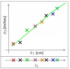
Figure: Dimensionality Reduction

Source: https://www.analyticsvidhya.com/blog/2015/07/dimension-reduction-methods/
The above graph represents two measurements x₁ and x₂ of the size of objects, measured in centimeters and inches. These measurements, if used to train a model, will cause unnecessary noise due to redundancy. Thus, the two-dimensional data is converted into one measurement z₁ which makes it easy to understand the data.
See also,
Principal Component Analysis (PCA)

Distance-based Clustering

Distance-based clustering is a method of segregating data points into clusters depending upon the distance between them. It is based on the idea that data points closer in data space are mutually more similar to each other than those lying farther away.
There are two approaches to distance-based clustering. In the first approach, data points are classified into separate clusters, and then they are aggregated, as the distance between clusters decreases. In the second approach, all data points are classified as a single cluster, and then they are partitioned, as the distance increases.

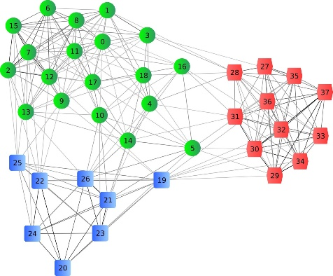
Figure: Distance-based clustering

See also,
Data Clustering

Durbin Watson Test

Durbin Watson test is used to measure the presence of autocorrelation (or serial correlation) at lag 1 between the residuals in statistical regression analysis.
The Durbin Watson test looks for a specific type of serial correlation called the AR(1) process.
The hypotheses for the Durbin Watson test are:

• H₀ = no first order autocorrelation
• H₁ = first order autocorrelation exists

The assumptions for the Durbin Watson test are:

• The errors are normally distributed with a mean equal to zero (0).
• The errors are stationary.

The Durbin Watson test statistic DW is:

DW=t=2Tet –et–12t=1Tet2

Where,
e_t and e_t–1 = residuals from an ordinary least squares regression.

The value of the Durbin Watson statistic always lies between 0 and 4.

Table: Values of DW statistics and their Interpretation

For example, stock prices tend to have a serial correlation because they do not change radically on a day-to-day basis. Thus if there is a positive autocorrelation between stock prices yesterday and today, a rise in prices yesterday would mean that the prices are likely to rise today. On the other hand, if stock prices display a negative autocorrelation, a rise in prices yesterday would mean that the prices are likely to fall today.

False Positive Rate

False positive rate is the probability in any test or ML models of falsely rejecting the null hypothesis.
It is quantitatively measured as the false positive ratio (FPR) given by
FPR = FP / (FP + TN)
Where,
FP = number of false positives
TN = number of true negatives
FP + TN = total number of negatives
See also,

• Confusion Matrix
• False Positive
• True Negative
• True Positive
• False Negative

Fit intercept

Fit intercept is a Boolean parameter in scikit-learn's linear regression algorithm. We can specify whether we want to include an intercept in the model or not. It has two values, True and False.
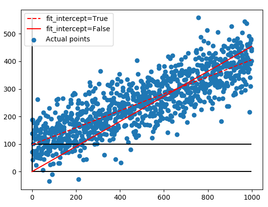
By default, the value is set to True. It means that sklearn automatically includes an intercept in the calculations. The y-intercept is determined by the line of best fit, which also fits the y-axis to the most suitable location (close to 100 in the graph below)
If the value is set to False, the model forcefully sets the y-intercept at the origin (0,0).

Figure: Fit intercept

F-score

In binary classification, F-score (also called the F-measure or F₁ score) is a measure of the accuracy of a test. It is the harmonic mean of the precision and the recall of the test.
It is calculated as,
F-score = 2 (precision × recall) / (precision + recall)
Where,
precision = positive predictive value, which is the proportion of the positive values that are positive
recall = sensitivity of a test, which is the ability of the test to correctly identify positive results to get the true positive rate.
The best F-score is 1 where the test delivers the perfect precision and recall, while the worst F-score is 0 which indicates the lowest precision and lowest recall.
See also,

• Receiver Operating Characteristic (ROC) Curve
• Specificity
• True Positive Rate
• Lift Chart

F-test of significance

The F-test of overall significance is a statistical test that indicates whether the linear regression model fits the data better as compared to a model that contains no independent variables (also called the intercept-only model).
The F-test is designed to test if two population variances are equal or not. It does this by comparing the ratio of two variances. The F-test is calculated using the formula
F= s12s22
Where,
s₁² and s₂² = sample variances
F-test is very flexible as it can be used in a variety of settings. It can evaluate multiple terms in a model simultaneously and compare the fits of multiple linear regression models.
F-test works on two hypotheses given below:

• The null hypothesis, according to which the intercept-only model fits the data as well as your model.
• The alternate hypothesis, according to which your model fits the data better compared to the intercept-only model. In inferential statistics, we can find the overall F-test value in the ANOVA table.

See also,
Analysis of Variance (ANOVA)

Geo-mapping

Geo-mapping is a data visualization technique of converting raw data into a country, continent, or region map. It makes it easier to understand and interpret data.
Simple pin map, heat map, territory map, and bubble maps are some types of geo maps.

Figure: Bubble geo map

See also,
Data Visualization

Heat Map

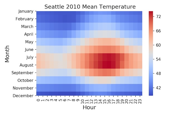
A heat map is a graphical visualization of data which depicts values as colours in two dimensions. It gives the observer a visual cue about how a phenomenon is clustered or how it varies over a given space. This is done by varying colours based on hue or intensity.

Figure: Typical heat map

See also,
Data Visualization

Hypothesis Test

Hypothesis testing is an act in statistics whereby an analyst tests an assumption regarding a population parameter. The methodology employed by the analyst depends on the nature of the data used and the reason for the analysis.
Hypothesis testing is used to assess the plausibility of a hypothesis by using sample data. Such data may come from a larger population, or from a data-generating process. The word "population" will be used for both cases in the following descriptions.

Incremental Learning

Incremental learning is a machine learning algorithm that uses new input data to train the model continuously and enrich its knowledge. It is used when the training data is available periodically, or the data size is beyond the limit of system memory.
This algorithm processes the data, taking one element at a time. They store a small number of elements like a constant number.
Incremental learning algorithms are weaker than batch algorithms (In batch learning, you have a set of train data called 'batch'. Batch learning trains your algorithm once using this complete set of train data) in their ability to detect clustering structure.
See also,

• Data Clustering
• Centroid-based Clustering
• Connectivity-based Clustering
• Density-based Clustering

Independent Variable

Independent variable (also called predictor/input/x variable) is an attribute whose variation decides the change in the value of another attribute of data, which is the dependent variable (also called the output/outcome/target variable or response).
In any experimentation, the value of the independent variable is altered and its effect on the dependent variable is studied.
In the linear equation y = mx + c, y is a dependent variable that depends on the independent variable x.
For example, if you study the impact of the number of study hours (x) of a student on the percentage of marks (y) in the examination, then y is the dependent variable, and x is the independent variable.
See also,
Dependent Variable

k-Nearest Neighbor

The k-nearest neighbour is a simple and easy-to-use supervised machine learning (ML) algorithm that can be applied to solve regression and classification problems. It assumes that similar things (for example, data points with similar values) exist in proximity. It combines simple mathematical techniques with this similarity to determine the distance between different points on a graph.
The input consists of k number of closest training examples in the feature space. The output, which is a class membership, depends on whether the algorithm is being used for regression or classification. In the case of regression, the mean of k labels is returned, while in case of classification, the mode of k labels is returned.
The object is classified by a majority vote of its neighbors, with the object being assigned to the class among its k nearest neighbors.
See also,
Regression

Kurtosis

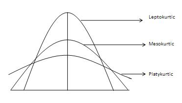
Kurtosis, in probability theory, is the measure of the tailedness of a data distribution compared to the normal distribution. It defines how much a given data is outlier prone. Kurtosis identifies whether the tails of a given distribution contain extreme values.
If a given data distribution has high kurtosis, it is heavily tailed and has outliers. On the other hand, the data distribution with low kurtosis is lightly tailed and lacks outliers. In the figure below, the mesokurtic curve is normal, the leptokurtic curve is more outlier-prone, while the platykurtic curve is less outlier-prone.

Figure: Types of kurtosis curves

Source: https://www.tutorialspoint.com/statistics/kurtosis.htm
See also,

• Skewness
• Descriptive Statistics
• Standard Deviation

Lasso Regression

Lasso stands for Least Absolute Shrinkage and Selection Operator. It is a regression analysis method that uses shrinkage to perform both variable selection and regularization in order to increase the prediction accuracy and interpretability of a statistical model.
Shrinkage refers to the fact that the data values shrink towards a central point, like the mean. Lasso regression performs L1 regularization in which a penalty equal to the absolute value of the magnitude of coefficients is added. In this case, some coefficients become zero and are eliminated from the model. Also, heavy penalties result in coefficients with values close to zero. This produces simpler models that are easy to analyse.
Thus, Lasso regression encourages simple and sparse models, where models have a less number of parameters. It is suitable for models that show great collinearity, to automate variable selection or parameter elimination in a model selection.
See also,
Regression

Likelihood (Conditional Probability)

The likelihood (also called conditional probability) of an event is defined as the probability of the occurrence of an event when another event has already occurred.
For example, a box contains 4 silver coins and 6 gold coins. Suppose one gold coin has been drawn. Then, the likelihood of drawing a second gold coin again will be
P = (6/10) × (5/9) = 30/90 = 1/3
Quantitatively, the likelihood of an event B when event A has already occurred (also called B given A) is defined as the ratio of the probability of event A and event B and the probability of event A.
P (B ǀ A) = P (A and B) / P (A)
See also,

• Probability
• Log of Odds (Log Odds)

Linear Regression

Linear regression is a statistical as well as machine learning (ML) method to establish a linear relationship between the input variables and a single output variable. The value of y can be calculated from linear combination of variables x.
The output variable is the dependent variable or scalar response, while the input variables are independent or explanatory variables.
There are two types of linear regression, simple and multiple. In simple linear regression there is only one input variable, while in multiple linear regression there are multiple input variables.
The aim of linear regression is to determine, which predictors are significant in predicting the output variable, their efficiency in predicting the output variable, and how do they impact the output variable.
See also,
Regression

Log of Odds (Log Odds)

In logistic regression, the log of odds (also called log odds) is a way of determining the probability. It is measured by taking the natural logarithm of the odds ratio. An odds ratio of an event is the ratio of the probability of success to the probability of failure. Then, the log of odds is the natural logarithm of this ratio.

Log Odds = Ln \[p / (1 - p)\]

Where, Ln = natural logarithm p = probability of an event happening 1 – p = probability of an event not happening For example, today there is an 80% probability of the day being a sunny day. It also means that there is a 20% probability of the day being cloudy. Thus, log odds of a sunny day are, Log odds = Ln (80/20) = Ln (4) = 1.386

See also,

• Probability
• Likelihood (Conditional Probability)

Mean

Mean, or the arithmetic average, is a measure of the central tendency of a finite set of discrete values in a dataset. It is calculated by adding the values and then dividing it by the total number of values.
See also,

• Median
• Mode
• Standard Deviation
• Descriptive Statistics
• Variance

Mean Square (MS)

In the ANOVA table, the mean square is an indicator of the variance of a population. It is measured by dividing the sum of squares by the degree of freedom.
In regression analysis, MS is used to determine whether the terms in the model are significant or not.
See also,
Analysis of Variance (ANOVA)

Median

Median is a measure of central tendency of a finite set of discrete sorted values. It is the middle number of that set arranged in the ascending or descending order.
Thus, median is more descriptive as compared to the arithmetic mean as it is higher half of the data sample from the lower half. It is applied more frequently compared to mean in cases where there are more outliers in the datasets, which might skew the average of these values.
See also,

• Mean
• Mode
• Standard Deviation
• Descriptive Statistics
• Variance

Mean Square (MS)

Multilayer Perceptron (MLP) is a class of artificial neural networks. A perceptron is an algorithm used for binary classification, which means that it predicts whether the input belongs to a certain category of interest or not.
See also,
Regression

Mode

Mode is a measure of the central tendency of a finite set of discrete values in a dataset. It is the value that appears most often in the set.
Among all the measures of central tendency, the mode is the least used and can only be used when dealing nominal data.
A data set may be unimodal (containing one mode), bimodal (containing two modes), or even multimodal (containing multiple modes).
See also,

• Mean
• Median
• Standard Deviation
• Descriptive Statistics
• Variance

Multinomial Logistic Regression

Multinomial logistic regression, also called as the Softmax regression, is a supervised ML algorithm applied to multiclass problems like text classification.
It is similar to the linear regression model, only with the difference that the linear regression model is generalized to classification problems that have more than one outcome.
It is used to predict the probability of different possible outcomes of a categorically distributed dependent variable.
See also,

• Regression
• Binomial Logistic Regression

MySQL

MySQL is a free and open-source relational database management system written in C and C++.

Naive Bayes

The Naive Bayes algorithm is a classification algorithm based on Bayes theorem. It assumes that the predictors are independent of each other.
The Naive Bayes classifier assumes that the presence of a feature in a class is independent of the presence of any other feature.
See also,
Data Classification

Network Diagram

Network diagrams (also called Graphs) show the interconnections between a set of entities. Each entity is represented by a Node (or vertice). The connections between nodes are represented through links (or edges).

No SQL

No SQL, also written as Non SQL or Not Only SQL, refers to a non-relational database. It means that these databases are used for the storage and retrieval of data in formats other than relational tables.

One sample proportion test

One sample proportion test is a hypothesis test used to estimate the proportion of one specific outcome in a population which follows the binomial distribution with a specific proportion.
It is based on certain assumptions like

• simple random method is used for sampling
• each sample point can result into only two outcomes which are 'success' and 'failure'
• the sample has at least ten successes and ten failures, and
• the population size is at least 20 times bigger than the sample size

See also,

• One sample t-test
• One sample z-test

One sample t-test

One sample t-test is a hypothesis test used to determine whether the sample mean is statistically different from the known mean or the hypothesized population mean.
One sample t-test can be based on two hypotheses, the null hypothesis, and the alternative hypothesis. The null hypothesis assumes that there is no difference between the true mean and the comparison value, whereas the alternative hypothesis assumes that a difference exists between the two.
In case of null hypothesis, the purpose of one sample t-test is to find out whether we can reject the null hypothesis in a given sample data.
In the case of alternative hypothesis, the purpose is to find out whether

• the difference between true mean and comparison value is non-zero (two-tailed hypothesis)
• the true mean is greater than the comparison value (upper-tailed hypothesis) or
• the true mean is smaller than the comparison value (lower-tailed hypothesis)

See also,

• One sample proportion test
• One sample z-test

One sample z-test

One sample z-test is used to determine whether the mean of a population is greater than, less than, or not equal to some hypothesized value. It is called one sample z-test because the normal distribution of the population is used to find the critical values in the test. The z-test assumes that the standard deviation of the population is known.
Like the one sample t-test, this test is also based on null and alternate hypotheses.
The standard score or the z-score gives an idea as to how many standard deviations above or below the population mean the individual raw score is. The z-scores range from -3 standard deviations to +3 standard deviations on the normal distribution curve. A zero z-score means that the value is exactly equal to the mean.
See also,

• One sample proportion test
• One sample t-test

Outlier Detection

Outlier or anomaly detection is the process of finding data objects that exhibit behaviour significantly different from the expected behaviour. Such data objects are called outliers or anomalies.
Outliers can be a serious issue while training ML algorithms or implementing statistical techniques. They arise because of some errors in measurement or some exceptional system conditions that produce abrupt changes in measurement.
Thus, best practices suggest a detection and removal of outliers from datasets. However, in some cases, outlier detection might prove to be valuable to highlight the anomalies that exist in the entire system.
See also,
Box Plot

Pearson coefficient

Pearson coefficient is a statistical constant that is used to measure the linear correlation between two variables.
It is also called Pearson's r or bivariate correlation or Pearson product-moment correlation coefficient.
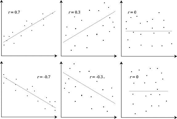
The value of Pearson's coefficient lies between -1 and +1. The zero value of Pearson's coefficient indicates no linear correlation.

Figure: Positive, negative and zero Pearson's r

Source: https://statistics.laerd.com/statistical-guides/pearson-correlation-coefficient-statistical-guide.php
See also,
Correlation

PostgreSQL

PostgreSQL is a general-purpose object-relational database management system. It is free and open-source software.

Probability

In statistics, the probability is the likelihood (or chance) of the occurrence of an event in a random experiment. Higher the probability, more likely is the event to occur.
Quantitatively, the probability of any event lies between 0 and 1. The value 1 indicates that the event is certainly possible while the value 0 means that the event is impossible.
See also,

• Log of Odds (Log Odds)
• Likelihood (Conditional Probability)

p-value

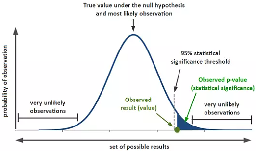
In statistics, the p-value (or the calculated probability) is the probability of obtaining the observed results, or more extreme, of a hypothesis test, assuming that the null hypothesis of the study question is true.
The p-value is compared with the significance level to check whether the data supports the null hypothesis or alternate hypothesis.
If the p-value is less than the significance level, the null hypothesis is rejected. It means that there is a significant difference between the true population parameter and the null hypothesis value. Thus, there is strong evidence in favor of the alternate hypothesis.

Figure: Location of p-value

Principal Component Analysis (PCA)

Principal Component Analysis (PCA) is a technique of dimensionality reduction which is used to find out the principal components in a dataset.
It reduces the number of variables by eliminating the redundant ones (retains only relevant variables) and improves the interpretability of the dataset. It also makes sure that there is minimum information loss and at the same time maximum retention of variability.
Thus, PCA makes the data easy to explore and visualize. Since it highlights variability, it is also helpful in bringing out the strong patterns in a dataset.
PCA computes a new set of variables called the 'principal components' and expresses the data in terms of these new components. These new variables express the same amount of data so much so that the original dataset is restored in a new form.
The total variance remains the same. However, it is unequally distributed among the principal components. The first principal component individually explains the maximum variance. Under certain restrictions, the first k principal components explain the most variance while the last k explain the least variance.
The fraction of the variance explained by any principal component is the ratio of the variance of that component to the total variance.
See also,
Dimensionality Reduction

Random Forest

Random forest is a flexible and easy-to-use ML algorithm for classification that gives excellent results even without the use of hyperparameters. It builds and then merges multiple decision trees to deliver a more accurate and stable prediction.
It is a supervised algorithm which contains a multitude of decision trees which are usually trained using the bagging method. The idea behind the bagging method is that a combination of learning models increases the overall result. The output of random forest technique is the mode of the classes, and it rectifies the overfitting habit of decision trees to the training dataset.
See also,

• Data Classification
• Decision Tree

Random Sampling

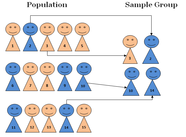
Random sampling is a technique of sample selection in which each element of the dataset has an equal probability/chance of getting chosen.
Random sampling is one of the simplest methods of data selection. It is very popular because it is considered to be an unbiased representation of the population. However, there might be a sampling error owing to variation in representation.

Methods like lotteries or random draws are used in random sampling.

Figure: Random selection of elements

See also,
Stratified Sampling

Random Seed

In Python, a random function is used to generate random numbers for some values. These are pseudo-random numbers in reality because they can be determined. The value for which these numbers are generated is called the seed value.
Seed value saves the state of a random function. Thus, when a code is executed multiple times on the same machine or different machines, the random function generates the same random number.

Regression

Regression is a statistical method, used in finance, investment, and other disciplines, that attempts to determine the strength and character of the influence of one or more independent variables on a dependent variable.
Regression helps investment and financial managers to value assets and understand the relationships between variables, such as commodity prices and the stocks of businesses dealing in those commodities.
See also,

• Binomial Logistic Regression
• Linear Regression
• Lasso Regression
• Multinomial Logistic Regression
• Ridge Regression

Ridge Regression

Ridge regression is a fundamental regularization technique that is used to analyze multiple regression data, which is multicollinear. It creates parsimonious models in the presence of a large number of features.
Multicollinearity occurs when independent variables (or predictors) in a regression model are correlated. This correlation is a matter of concern because predictors should be independent. If the degree of correlation between predictors is high enough, it can cause issues when you fit the model and interpret the results.
Ridge regression is used to regularize the coefficients in a model so that their value is pushed close to zero. When the values of coefficients are close to zero, the models work better on new datasets optimized for prediction.
Ridge regression performs L2 regularization in which a penalty equivalent to the square of the magnitudes of the coefficients is added. This addition of penalty minimizes the error between the actual and the predicted observations.
See also,
Regression

Root Mean Square Error (RMSE)

Root Mean Square Error (RMSE) is the standard deviation of the residuals. It is a standard way to measure the error of a model in predicting quantitative data.
RMSE is used to serve as a heuristic for training models and to evaluate trained models for usefulness/accuracy.
When we perform any regression analysis, we get a line of best fit (also called the regression line). But all data points do not lie exactly on the line; they are scattered around it. Residual is the vertical distance of a data point from this regression line. Thus, residual, and in turn, RMSE, is a measure of the concentration of data around a regression line.

Sensitivity

Same as True Positive Rate.
See also,

• Receiver Operating Characteristic (ROC) Curve
• Specificity
• True Positive Rate
• Lift Chart
• F-score

Shapiro-Wilk Normality Test

The Shapiro-Wilk test is a normality test in probability determination statistics. It is used to find out whether a random sample has been derived from a normal distribution.
The Shapiro-Wilk test for normality is one of the three general normality tests designed to detect all departures from normality. It is comparable in power to the other two tests, that is the Durbin-Watson test and the Anderson-Darling test.
The test rejects the hypothesis of normality when the p-value is less than or equal to 0.05. Failing the normality test allows you to state with 95% confidence that the data does not fit the normal distribution. Passing the normality test allows you to state that no significant departure from normality was found.
The test generates a W value which depends on the ordered random sample values and the constants generated by covariances, variances, and means of a normally distributed random sample. If the W value is small, the null hypothesis is rejected and it can be concluded that the random sample is not normally distributed.
Shapiro-Wilk normality test generates a significant result if the sample size is sufficiently large.

Significance Level (α)

The significance level (α) (also called the Type I error) is the probability of rejecting the null hypothesis when it is true. The value of α lies between 0 and 1.
If the power of test (1 – β) is too small, one should consider high value of α like 0.1, 0.2, 0.5, and so on.
For example, if α = 0.05, it indicates that there is a 5% probability of difference existing between the population parameter and the null hypothesis value, whereas there is no such difference (null hypothesis).

Skewness

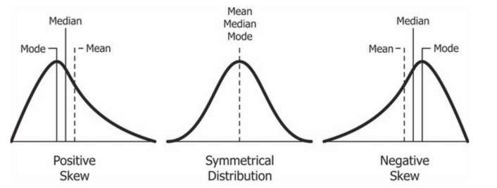
Skewness refers to the distortion or the asymmetry in a symmetrical bell curve or normal distribution in a dataset. A skewed curve is shifted either to the left (negative) or to the right (positive). A curve with zero skew is normally distributed.
Skewness is a measure of the asymmetry of the probability distribution of a real-valued random variable about its mean. The skewness value can be positive, zero, negative, or undefined. Skewness focusses on the extremes of a dataset rather than concentrating on the average.

Figure: Positive and negative skewed curves

See also,

• Mean
• Median
• Mode
• Variance
• Kurtosis
• Descriptive Statistics
• Standard Deviation

Specificity

In binary classification, specificity (also called inverse recall) represents the proportion of negative results that were correctly classified. It is the ratio of the correctly classified negative samples to the total number of negative samples.
It is quantitatively measured as
Specificity = TN / (TN + FP)
Where,
TN = number of true negatives
FP = number of false positives
See also,

• Confusion Matrix
• False Positive
• True Negative
• True Positive
• False Negative
• Receiver Operating Characteristic (ROC) Curve
• True Positive Rate
• Lift Chart
• F-score

Standard Deviation

Standard deviation is a statistical term that measures the dispersion of a dataset relative to its mean. If standard deviation is high, the data is more spread out, that is, the data points are more spread out in the distribution.
Standard deviation is measured as the square root of the variance.
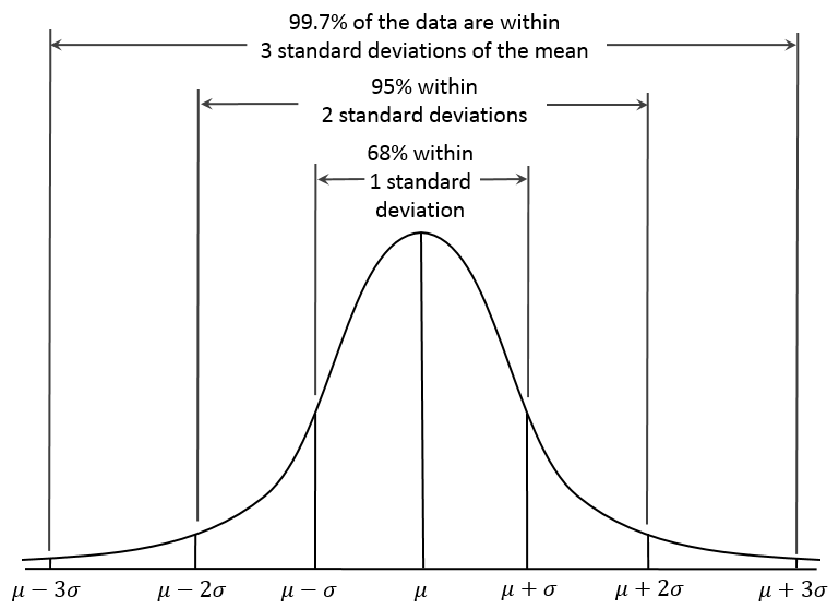
The graph shown below represents a normal distribution curve. For datasets that represent normal distribution, standard deviation is used to determine the percentage of values that lie within a particular range of the average value. In this case,

• Almost 68% values are less than 1 SD away from the mean value
• Almost 95% values are less than 2 SD away from the mean value
• Almost 99.7% values are less than 3 SD away from the mean value

Figure: Standard deviation curve

See also,

• Mean
• Median
• Mode
• Descriptive Statistics
• Variance
• Kurtosis
• Skewness

Standardized Residuals

Standardized (or simply standard) residual is a measure of the strength of the difference between observed and expected values.
Standard residual is measured as a ratio of the residual (the difference between the observed and expected count) and the standard deviation of the expected count in the chi-square testing.
Standardized residuals express the magnitude of residuals in units of standard deviation. Hence, it becomes easy to identify outliers in a sample.

Stratified Sampling

Stratified sampling is a method in which the population is divided into separate groups called strata. Then, the probability sample (usually a simple random sample) is drawn from each of these strata.
Stratified sampling technique has several advantages over random sampling. Stratified sampling can reduce the sample size required for a given level of precision, or it may give a higher precision with the same sample size.
See also,
Random Sampling

Sum of Squares (SS)

In the ANOVA table, the sum of squares is the sum of the square of the variations. Variation is the difference (or spread) of each value from the mean.
First, the distance of each data point from the line of best fit (or regression line) is determined. Then all these distances are squared and added to give the sum of squares. The line of best fit gives a minimum value of SS.
See also,
Analysis of Variance (ANOVA)

Threshold Value

Predictive models in binary classification are capable of class labeling. This means that they can decide the class of a variable as 0 or 1, True or False, Positive or Negative, and so on.
To map the logistic regression value to a binary category (0 and 1), we define a classification threshold or decision threshold. This threshold value is problem-dependent.
For example, 0.5 is the threshold of a classification problem. It means that any predicted value below 0.5 is classified as zero (0), while any predicted value greater than or equal to 0.5 is classified as one (1).

True Positive Rate

In binary classification, a true positive rate (also called sensitivity or hit rate or recall) is the ability of a test to correctly identify the positive results. Thus, it is the ability to test positive where the actual value is also positive.
It is quantitatively measured as the true positive ratio (TPR) given by
TPR = TP / (TP + FN)
Where,
TP = number of true positives
FN = number of false negatives
See also,

• Confusion Matrix
• False Positive
• True Negative
• True Positive
• False Negative
• Receiver Operating Characteristic (ROC) Curve
• Specificity
• Lift Chart
• F-score

Two independent samples t-test

Two independent samples t-test is an inferential statistical test that is used to determine the statistical difference between the means in two unrelated groups.
Two independent samples t-test needs one independent categorical variable that has two levels and one continuous dependent variable. Unrelated groups are those in which cases or participants are different.
See also,

• Two paired samples t-test
• Two sample z-test
• Two samples proportion test

Two paired samples t-test

Two paired samples t-test (or the dependent samples t-test) is a statistical technique in which we check whether the mean difference (MD) between the two sets of observations (we take before-after data is used) is zero. Thus, the samples are not independent.
In this test, each subject is measured twice, thus giving pairs of observations.
Two competing hypotheses are constructed for this test. These are the null and alternate hypotheses. The null hypothesis assumes that the mean difference between the paired samples is zero. The alternate hypothesis can be upper-tailed (MD > 0), lower-tailed (MD < 0), or two-tailed where MD is not equal to zero.
This test is used in case-control studies or repeated-measures designs.
See also,

• Two independent samples t-test
• Two sample z-test
• Two samples proportion test

Two sample z-test

A two sample z-test is a statistical test used to determine whether the two population means are different when the variances are known, and the sample size is large.
For an accurate z-test, it is assumed that the data is normally distributed and the standard deviation is known. A z-score indicates how many standard deviations above or below the mean population a z-test score is.
See also,

• Two independent samples t-test
• Two paired samples t-test
• Two samples proportion test

Two samples proportion test

Two sample proportion test or the z-score test is used to determine whether two populations or groups differ significantly on some categorical characteristic.
This test is used when the sampling method used for each population is simple random sampling and the samples are independent. Each sample includes at least 10 successes and 10 failures. This test has a null hypothesis that there is no difference between the two population proportions.
See also,

• Two independent samples t-test
• Two paired samples t-test
• Two sample z-test

Variance

Variance is a statistical measure of the extent of spreading of a dataset. It is measured as the average square deviation of each number in the data set from its mean.
It measures how far a set of numbers are spread out from their average value.
See also,

• Mean
• Median
• Mode
• Descriptive Statistics
• Kurtosis
• Skewness

Variance Inflation Factor

The Variance Inflation Factor (VIF) is used to detect multicollinearity in regression analysis.
Multicollinearity refers to the presence of correlation between various predictors (independent variables) in an analysis, which affects the regression results adversely. VIF measures the inflation of the regression coefficient due to multicollinearity.
VIF is calculated by selecting one predictor and regressing it against all other predictors in the model. This generates the R² value which is then used to calculate VIF. The decimal part in the value of VIF indicates the percentage of variance inflation for each coefficient. For example, a VIF of 1.6 means that the variance of a coefficient is 60% bigger than what it would be in the absence of multicollinearity.
The value of VIF is equal to or greater than 1. If VIF = 1, the predictors are not correlated. If VIF is between 1 and 5, they are moderately correlated. For any value greater than 5, the predictors are heavily correlated. Higher the value of VIF, lower is the reliability of the regression results, and ultimately the model.