Advanced Entity Extraction
Advanced entity extraction, also known as entity recognition, is used to extract vital information for natural language processing (NLP). It is widely used for finding, storing and sorting textual content into default categories such as person, locations, objects, organizations and so on.
Thus, advance entity extraction involves identification of proper names in texts and their classification into a set of predefined categories of interest.
See also,
rubitext
Algorithm
Algorithm is a step-by-step procedure to solve logical and mathematical problems. It takes an input and produces a logical output.
Algorithms contain an ordered set of rules or instructions which determine how a certain task is accomplished in order to achieve the expected outcome.
Algorithms can be written in any ordinary language (for example, writing the steps for a recipe). However, in computing, algorithms are written in pseudocode, flowcharts or a programming language.
See also,
Machine Learning Algorithms
ARIMA
ARIMA stands for Autoregressive Integrated Moving Average model. It is fitted to the time-series data to understand the data better, or to predict the future data points in the series based on its own past values.
ARIMA is based on the assumption that only the information in the past values of a time-series data can be used to predict its future values. Thus, it is a univariate time-series forecasting model.
ARIMA is made up of three components – AR (past values used to forecast the next value), I (number of times the differencing operation is performed on the series to make it stationary), and MA (number of past forecast errors used to forecast the next value). However, in some cases, ARIMA models are applied where data shows evidence of non-stationarity. In that case, an initial differencing step can be applied one or more times to eliminate the non-stationarity.
ARIMA models are used in short-term non-seasonal forecasting and require a minimum of 40 historical data points.
See also,
Auto ARIMA
In ARIMA, before implementing the forecasting model, data preparation and parameter tuning are complex and time-consuming. It is necessary to make the model stationary and determine the values of AR (Autoregressive) and MA (Moving Average), before the model is actually implemented.
Auto ARIMA makes the implementation of the ARIMA model easier by performing all data preparation and parameter tuning operations. It makes the series stationary and determines the values of the three coefficients of ARIMA, by creating Auto Correlation Function (ACF) and Partial Correlation Function (PACF) plots.
See also,
Basic Sentiment Analysis
Basic sentimental analysis is the mining of textual data to extract subjective information from the source. This helps businesses to understand the social sentiment about their product, service, or brand based upon the monitoring of online conversations.
In this analysis, the algorithm treats a text as Bag of Words (BOW), where the order of words and their context is ignored. The original text is filtered down to only those words that are thought to carry sentiment. Also, the algorithm keeps count of the maximum number of occurrences of the most frequent words.
Sentiment analysis models focus on polarity, that is, they detect whether the text evokes a positive, negative, or neutral sentiment. Apart from this polarity, these models can also detect emotions, feelings (for example, happy, sad, disappointed, or angry), and intentions (for example, interested or not interested).
Table: Sentiment Scores and their Meaning
Sentiment | Sentiment Score | Remark |
Positive | 0.01 to 1 | 0.01 is the weakest sentiment score, while 1 is the strongest sentiment score. |
Negative | -0.01 to -1 |
|
Neutral | 0 | Neutral statement |
See also,
Case Convertor
Case convertor can change the case of an alphabet from an upper case to a lower case or vice-versa.
See also,
Centroid-based Clustering
Centroid-based clustering is a method in which each cluster is represented by a central vector. The central vector may not necessarily be a part of the dataset. A data value is assigned to a cluster depending upon its proximity, such that its squared distance from the central vector is minimized.
The k-means algorithm is the most widely used centroid-based clustering algorithm. In this algorithm, the dataset is divided into k pre-defined, distinct, and non-overlapping clusters. Each data point is assigned to a cluster such that the arithmetic mean of all data points within a cluster is always minimum. Minimum variation within a cluster ensures greater homogeneity of data points within that cluster.
See also,
Incremental Learning
Connectivity-based Clustering
Connectivity-based clustering is also called hierarchical clustering. This is because it builds clusters in a hierarchy. In clustering, the data points that are closer to each other exhibit more similarity than those which are away from each other.
The algorithm starts with assigning of data points to a cluster of their own. Then two nearest clusters are merged to form a single cluster. In the end, the algorithm terminates with only one cluster remaining.
There are two approaches to this model. In the first approach, data points are classified into separate clusters and then aggregated as the distance between them decreases. In the second approach, data points are distributed into a single large cluster and then segregated as the distance between them increases.
See also,
Custom Words Remover
One of the major tasks of data pre-processing is to filter out unnecessary data. In Natural Language Processing (NLP), words that are filtered out from the text are called stop words. Stop words are usually the most common words in the language. For example, 'the', 'is', 'of', 'to', 'in', and so on are regarded as stop words in English. However, all NLP tools do not use the same list of universal stop words. Users can specify which stop words are to be removed.
Custom words remover eliminates the user-specified custom word/words before further processing. The output is a text without stop words.
See also,
Dashboard
A dashboard is a Graphical User Interface (GUI), which displays all the key performance indicators at a glance. In short, it is a progress report generated to gauge the performance of a process, business, and so on.
In rubiscape, a dashboard is an interactive platform hosted in rubisight, where the insights and outcomes of a successfully run model are displayed.
See also,
RubiSight
Data Aggregation
Data aggregation is a process in which information is collected and summarized in a specific form. It can be used for data analysis or statistical analysis.
The aim of aggregation is to derive additional information and insight about groups based on variables.
See also,
Data Preparation
Data Analysis
Data analysis is the investigation, cleaning, transforming, and modelling of data. It is useful to detect appropriate information, draw calculated conclusions, and support decision-making in businesses.
Data analysis includes diverse approaches and techniques used in many businesses, scientific explorations, and sociological studies. In today's business world, data analysis plays a vital role in making decisions more precise and scientific. In turn, this helps businesses to function more effectively.
See also,
Data Cleaning
Data cleaning (or cleansing) is a process of preparing data for analysis by searching and rectifying inaccurate or corrupt records in a database, dataset, or tabular data. In data cleaning, we identify missing, incorrect, irrelevant, inconsistent, wrongly formatted, and inaccurate portions of the available data. Such data may obstruct the smooth analytical process and may deliver inaccurate results.
Data coming from various sources may be manually modified by users, may carry errors and gaps in it. Hence it is essential to clean and optimize data. Data cleaning is not only used to erase such inaccurate data but to maximize the accuracy of a dataset.
In rubiscape, data cleaning is performed using data wrangling tools.
See also,
Data Filtering
Data filtering is a method of refining datasets. It includes removal of repetitive, irrelevant, and sometimes sensitive data and retaining data which is needed by the user for further analysis.
In data filtering, a smaller portion of the dataset is selected for viewing and analysis. This selection is made on the basis of a certain rule or logic.
Data filtering is very useful in the process of training and validating statistical models.
See also,
Data Preparation
Data Integration
Data integration involves the combination or merging of data from different sources.
Data source network, master server, and a client are the important components in data integration. The client requests for data from the master server, which extracts data from internal and external sources, unifies it into a single uniform dataset and supplies it to the client.
Although there are no prevalent processes of data integration, it predominantly includes the ingestion of data, data cleaning, ETL (Extraction, Transformation, and Loading) mapping, and data transformation.
Data integration enables analytics tools to produce effective, actionable business intelligence. It is crucial for commercial as well as scientific purposes where large volumes of data (big data) are processed and shared. See also,
Data Joiner
Data joiner is a method to join two tables. The SQL JOIN clause is used to join rows based on a related column that is present in two or more tables.
The types of data join are given below.
(Inner) Join: It joins two tables and returns records containing only the matching values in both the tables.
Left (Outer) Join: It joins two tables and returns all records from the left table and only the matched records from the right table.
Right (Outer) Join: It joins two tables and returns all records from the right table and only the matched records from the left table
Full (Outer) Join: It joins two tables and returns all records when there are matched records in either the left table or the right table.
Self Join: It is a regular type of join in which the table is joined with itself.
Figure: Types of Data Joins
See also,
Data Merger
Data Merger
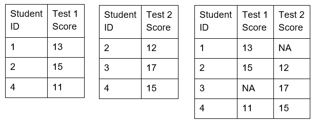
Data merger is a method to merge two or more rows to include them in a table. The rows of data appear one below the other in the resulting table. All the columns in the two tables (common or uncommon) are also retained in the resulting table.
Data merger is used to combine tables with similar data derived from different sources.
Generally, when we merge tables, there is a common element (a column with the same variable) in them. However, even if tables do not have identical columns, we can still merge them. The variable values for the absent columns in individual tables will be marked as 'na' in the combined table. Thus, neither the data is deleted nor omitted from the two tables.
Figure: Merging data from two tables
See also,
Data Joiner
Data Modeling
Data modeling is the process of creating a data model so that data can be stored in the database. A data model comprises of data objects, associations between data objects, and the rules.
Data modelling is a conceptual representation which stresses on the type of data required and the organization of data.
See also,
rubiML
Data Orchestration
Data Orchestration is a process in which data-driven processes are automated end-to-end. This includes data preparation, data processing, decision-making, and further taking necessary actions based on those decisions made.
Data orchestration contains a set of technologies that abstract data access across storage systems, virtualize the data, and present it through standard APIs with a global namespace to data-driven applications. Data orchestration is widely spread across various types, departments, and systems of data.
Data orchestration is crucial owing to the complexity of data ecosystems, new data frameworks, adoption and migration of data on cloud-based systems, and an increase in the number of data-driven applications.
See also,
Data Preparation
Data Preparation
Data preparation is the process of cleaning and transforming raw data into organized data so that it can be processed and analysed further. In data preparation, data is reformatted, corrected, and combined to enrich the data.
Data preparation is complex yet essential to create contextual data, so that the analysis of such data may prove efficient in producing reliable and insightful results. In the absence of preparation, biased data may result in poor analysis and erroneous results.
See also,
Data Preprocessing
Data Preprocessing
Data preprocessing is a data mining technique to transform raw data into useful formats.
It involves data cleaning, data transformation, and data reduction.
See also,
Data Scaling
Data scaling or feature scaling is one of the steps of data preprocessing applied to continuous independent variables or data features.
Data scaling limits the range of variables present in a data so that the variables become comparable on similar grounds. It normalizes data within a specified range. This helps to speed up of the algorithmic calculations.
See also.
Data Preprocessing
Data Science
Data science is an interdisciplinary field that employs scientific procedures, processes, algorithms, and systems to extract knowledge and insight from any type of data - structured or unstructured.
Data science combines the knowledge of statistical tools, business intellect, algorithms, and machine learning techniques to discover insights or patterns hidden in crude data to facilitate crucial business decisions.
Data science is all about finding current trends and patterns based on factual data so that they can be modelled and future conditions can be predicted.
See also,
Data Science Platform
Data science platform is a software nerve center or hub which provides a centralized and an all-inclusive location to perform all data science-related tasks. These tasks range from integrating and exploring data, coding and building models, deploying these built models into production, and generating useful results.
Each of these tasks requires specialized and diversified tools, and it becomes a challenge for data scientists to search for these tools in various places, organize them, and use them in coherence. A data science platform integrates all these tools and puts all the data modeling process in a single place. This makes the job of data scientists easier and faster. They can focus their attention on deriving insights from data analysis and conveying it to the decision-makers.
rubiscape is one such powerful, innovative, and comprehensive data science platform.
See also,
Data Sorting
Data sorting is the process of arranging the data in a purposeful and relevant order or sequence. This makes it easy to understand, analyse, and visualize data.
Data sorting is done based on data values, data counts or percentages. Data can be arranged in ascending or descending order. Data can also be sorted according to variable value labels. Value labels are nothing but metadata found in some programs which allow a researcher to store labels for each value option of a categorical question.
See also,
Data Preparation
Data Visualization
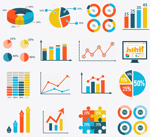
Data visualization is the representation of data in the form of pictures, images, graphs, or any other form of visual illustration. It allows decision makers in organizations to understand data analytics visually. This makes it easy for the user to understand the concepts that are complex, and identify new patterns easily.
Data visualization is both an art as well as a science. It involves a systematic alignment between graphical symbols and data values. This determines the visual representation of data. In other words, it represents the variation in data values with the help of the variation in the size and color of graphical symbols.
Figure: Various types of data visualization
Source: https://www.vectorstock.com/royalty-free-vector/infographic-set-graph-and-charts-diagrams-vector-4304313
See also,
rubisight
Dataset
A dataset is a compilation or collection of data, usually in the tabular form. However, non-tabular datasets can also be compiled, as in the case of an XML file, where data appears in the form of marked-up strings of characters.
In machine learning, data is mostly categorized into four types, namely numerical data, categorical data, time-series data, and textual data. However, there can be many other types of data depending upon the method of collection, tabulation, and so on.
In rubiscape, the datasets can be selected from a variety of dataset types like social media data, RDBMS data, File data, Hadoop data, API data, and Email data.
See also,
Reader
Decision Tree
A decision tree is a non-supervised machine learning tool or method used for regression and classification.
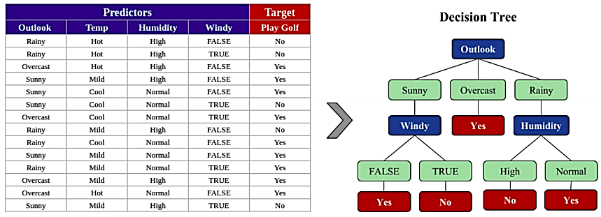
A decision tree builds a classification model like a tree structure. As the model develops, it breaks the dataset into increasingly smaller subsets. The result is a tree with decision nodes and leaf nodes. The structure has a single node called the root node at the top and further extends to decision nodes and leaf nodes, which are the classifiable categories.
The decision tree learns certain simple decision rules from data features. Using them, we develop a model that can predict the value of the target variable. Since decision trees are visual tools, they are easy to understand and interpret. They can manage multi-output problems and can predict using numerical as well as categorical data.
Figure: Converting data into a decision tree
Source: http://www.diva-portal.org/smash/get/diva2:1261957/FULLTEXT01.pdf
See also,
Density-based Clustering
Density-based clustering is an unsupervised learning method. It identifies distinctive clusters in data to be the regions of high point density, clearly separated from other clusters by a region of low point density. These separating regions of low point density are considered as noise or outliers.
In density-based clustering, core samples of high point density are identified, and clusters are developed from them. This method is suitable for data that contains data of comparable density. Also, clusters found in DBSCAN can be of any shape as opposed to the k-means method where clusters are assumed to be convex-shaped.
See also,
Exponential Smoothing
Exponential Smoothing is a time-series forecasting method for univariate data. In exponential smoothing, the prediction is a weighted average of the past observations, where the weight of an observation decays exponentially as the observation gets older. Thus, more recent observations have a higher associated weight, and older observations have a lower associated weight.
See also,
False Negative
A test result that wrongly indicates that a particular condition or attribute is absent can be termed as a False Negative result.
In terms of hypothesis testing, a false negative is a situation when you get a negative result and you do not reject a null hypothesis (when you actually should have rejected it). In other words, it is not rejecting a false null hypothesis. This is known as a Type II error.
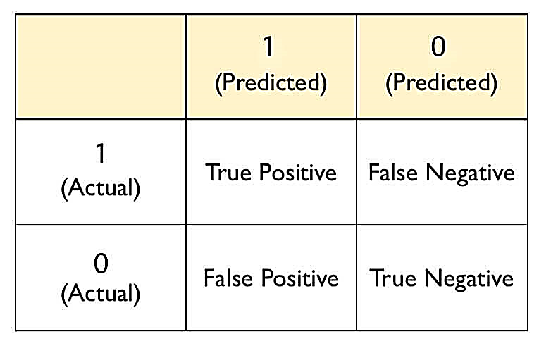
In the case of binary classification, a false negative is a situation where the predicted outcome is zero (0) whereas the actual outcome is one (1).
For example, a cancer detection test yields a negative result for a patient, whereas, in reality, the patient has cancer. In this case, the result is a false negative.
Figure: Predicted and Actual Values
See also,
False Positive
A test result which wrongly indicates that a particular condition or attribute is present (when in reality it is not) can be termed as a False Positive result.
In terms of hypothesis testing, a false positive is the rejection of a true null hypothesis. This is known as a Type I error.
In terms of binary classification, a false positive is a situation where the predicted outcome is one (1) whereas the actual outcome is zero (0).
For example, a cancer detection test yields a positive result for a patient, whereas, in reality, the patient does not have cancer. In this case, the result is a false positive.
Refer to the figure in the concept False Negative.
See also,
Frequent Words Remover
Frequent words remover is an algorithm that removes common words appearing in a given text input. This removes the plural forms of words and unnecessary repetition of nouns in a sentence. The output is a text free of frequent words.
See also,
Gradient Boosting
Gradient boosting is a powerful machine learning algorithm applied for regression and classification problems. It produces a prediction model, which is an assembly of weak prediction models, typically decision tree models. It builds models stage-wise and generalizes them by allowing optimization of an arbitrary differentiable loss function.
Gradient boosting works on the intuition that when the best possible next model is combined with the previous models, the error in overall prediction is minimized.
See also,
Holt Exponential Smoothing
Holt exponential smoothing is an extension of simple exponential smoothing, which allows the forecasting of data that has a trend but no seasonality. The forecast is made up of a level component and a trend component.
It involves one forecasting equation and two smoothing equations, out of which one is a level equation while the other is a trend equation.
See also,
Holt-Winters Exponential Smoothing
Holt-Winters exponential smoothing is an extension of the Holt exponential smoothing to include seasonality.
Holt-Winters exponential smoothing has two variations – the additive method and the multiplicative method.
Additive method is preferred when the seasonal variations are more or less constant throughout the series. The seasonal component is expressed in absolute terms in the scale of the observed series. The series is seasonally adjusted in the level equation by subtracting the seasonal component. Within each year, the addition of the seasonal component is approximately zero.
Multiplicative method expresses the seasonal component as a relative term, like percentage. The series is seasonally adjusted by dividing through by the seasonal component.
See also,
Hyperparameter
Hyperparameters (in machine learning) are parameters or characteristics whose value is set before starting the learning process. They are adjustable parameters that are chosen to train a model.
In ML, it is imperative to choose a model with an appropriate level of complexity. If a model is too complex, it will overfit the data but will not generalize properly to unseen data. On the other hand, if a model is less complex, it will underfit the data and will not be able to interpret all information in the data. Hyperparameters are used to solve this problem of overfitting and underfitting models.
Hyperparameters largely decide and influence the performance of a model in ML. Hyperparameter exploration is carried out to find out those hyperparameter configurations that help in tuning models so that we get the best-performing models.
Most of the common ML algorithms have a pre-defined set of hyperparameters.
Label Encoding
Label Encoder is a part of the scikit-learn library in Python and is used to convert categorical data or textual data into numerical data, which can be better understood and analysed by the predictive models.
For example, if a data column contains the name of countries or football teams, it cannot be interpreted by the model. Hence, numerical values are assigned to them. However, the algorithm may interpret that these assigned values are related to each other according to an order or a hierarchy. This is the drawback of label encoding and to overcome this drawback, One Hot Encoding is used.
See also,
One Hot Encoding
Lemmatizer
Lemma is a canonical/dictionary/citation form of a set of words. It takes into account the morphological analysis of words. For this, it is necessary to have a detailed dictionary that the algorithm looks through to link the form back to its lemma.
For example, the lemma of all the three words given below will be "Go".
Gone → Go
Going → Go
Went → Go
Lemmatizer is an algorithm that identifies the lemma (the root word or the dictionary form) of a word.
Unlike stemming, lemmatizer reduces the inflected words to a "root" word, ensuring that the root word is linguistically correct; that is, it also belongs to the language.
Lemmatization algorithms also identify the intended part of speech and the meaning of a word in a sentence in a broader context in the surrounding sentences and even in the entire document.
See also,
Lift Chart
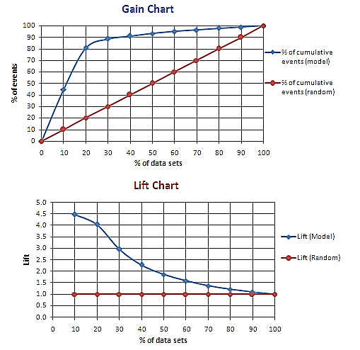
The lift chart serves as a visual aid in assessing the performance of a classification model.
A lift is the measure of the effectiveness of a model. It is the ratio of the percentage gain to the percentage of random expectation at a given decile level (Decile level is the quantitative method of splitting a ranked data into ten equal divisions). In other words, it is the ratio of the result obtained with a predictive model to that obtained without it.
A lift chart contains a lift curve and a baseline.
For example, a shopkeeper wants to contact his most loyal customers through telephone for advertising and selling a new commodity. The shopkeeper predicts a success rate of 20%. Thus, he expects that only 20% of those contacted would purchase the commodity.
In the lift chart below, the x-axis denotes the percentage of prospective customers contacted. The baseline (pink line) indicates the overall response rate. Thus, if X% of prospective customers are contacted, the shopkeeper will get X% of positive responses.
Also, in the lift chart below, the lift curve (blue line) denotes the percentage of positive responses obtained by contacting a given number of prospective customers. Thus, it is expected that the curve should go as high as possible towards the top-left corner of the graph.
Greater the area between the lift curve and the baseline, better is the model.
Lift charts are normally associated and drawn in tandem with gain charts.
Figure: Lift and Gain Charts
Source: https://www.listendata.com/2014/08/excel-template-gain-and-lift-charts.html
See also,
Machine Learning Algorithms
Machine learning algorithms are mathematical and logical programs which, when exposed to huge amount of data, can self-adjust to perform more efficiently and accurately. When an algorithm receives feedback on its previous output, it adjusts its parameters indigenously to perform better.
Thus, like humans, machines learn to modify themselves to process data over time.
Linear Regression, Logistic Regression, Random Forest, Neural Networks, and Naive Bayes classifiers are some of the most popular algorithms used in machine learning.
See also,
Machine Learning Models
Machine learning models are analytical and predictive models built using machine learning algorithms. They are consolidated form of machine learning algorithms which have been successfully trained, tested, and implemented.
See also,
rubiML
Maximum Entropy
The principle of maximum entropy is used while modeling a dataset. According to it, the most appropriate distribution is the one which has the highest entropy among all those distributions that satisfy the constraints of the prior knowledge. Thus, out of several probability distributions, the best choice is the one that has maximum entropy.
The maximum entropy classifier is a probability classifier which belongs to the family of exponential models. It does not assume that the features are conditionally independent of each other. It is extensively used in NLP, speech, and information retrieval problems such as language detection, topic classification, sentimental analysis, and many more.
See also,
rubitext
Missing Value Imputation
Many times, there are missing values in datasets. These datasets are incompatible for scikit estimators because these estimators assume that all values are meaningful numerical values. If we eliminate the rows in a dataset containing missing values, we may lose important and relevant data. Hence, missing value imputation fills the missing gaps by inferring the value from the known part of the data.
Missing value imputation can be univariate or multivariate. In univariate imputation, the missing value is replaced by a constant value or a statistical value like the mean or the median of the corresponding column. In multivariate imputation, each feature with missing value is modelled as a function of other features, and then this estimate is used for imputation.
See also,
Data Preparation
Normalization
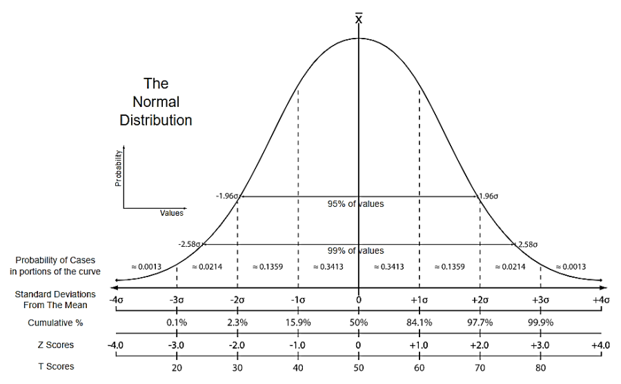
Normalization is used to change the data such that it can be represented as a normal distribution like a bell curve. In this case, the values are roughly equally distributed above and below the mean value. Also, the mean and the median are equal and maximum values are concentrated closer to the mean.
Figure: Normal Probability Curve (Bell Curve)
Source: https://kharshit.github.io/blog/2018/03/23/scaling-vs-normalization
See also,
One Hot Encoding
One hot encoding eliminates the confusion of a model in interpreting categorical data. It splits the column containing categorical data into multiple values and assigns them 0 or 1 as a value. This increases the number of columns in the table.
For example, if a column contains three football teams, namely X, Y, and Z, one hot encoder will split it into three columns. For the rows which have first column value as team X, the column for X will have 1, and the rest two values will have 0.
See also,
Label Encoding
Predictive Modeling
Predictive modelling is a technique that employs data models and uses statistical tools to predict outcomes.
Although predictive models cannot perform future analysis with 100% accuracy, they can predict the possible outcome.
See also,
rubicast
Punctuation Remover
Punctuation remover is an algorithm, used in textual analysis, to remove punctuation marks like a full stop, comma, semi-colon, question mark, exclamatory mark, and so on from the given text.
See also,
Random Walk
In statistics, a random walk is a process in which the movement of objects or values of a variable is entirely random, and there is no pattern or trend in it.
In random walks, each value in a sequence is a modification of the previous value in the same sequence. This model assumes that in each period, the variable takes a random step away from its previous value, and the steps are independently and identically distributed in size.
In random walk, objects wander away from where they started, the simplest example being the one-dimensional walk. Random walks and the mathematics that governs them are found everywhere in nature.
For example, when gas particles bounce around in a room, the change in direction that happens, every time they collide with another particle, is a random walk. The corresponding mathematics determines how long it will take the particle to travel from one location to another.
See also
Receiver Operating Characteristic (ROC) Curve
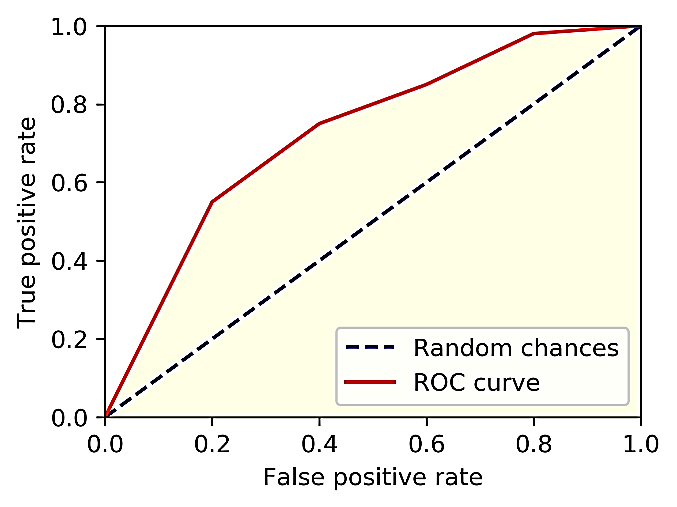
ROC curve is a probability curve that helps in the measurement of the performance of a classification model at various threshold settings. We can use ROC curves to select possibly the most optimal models based on the class distribution.
ROC curve is plotted with True Positive Rate (TPR) on the Y-axis and Error! Reference source not found. (FPR) on the X-axis.
The area under the curve (AUC) tells us how much the model can distinguish between the two classes. Higher the AUC, better is the model in predicting 0s as 0s and 1s as 1s. In the figure below, the dotted line is the random choice with probability equal to 50%, AUC equal to 0.5, and the slope equal to 1.
Theoretically, the AUC lies between 0 and 1. However, any meaningful classifier model should have an AUC greater than 0.5.
Figure: ROC Curve
See also,
Scaling
Scaling is the method of transforming data such that it fits within a specific range, like 0 to 1 or 0 to 100, and so on.
Scaling is used in the case of algorithms like Support Vector Machine or the k Nearest Neighbor, where we want to determine how much apart the data points are located.
See also,
Normalization
Sentiment
A sentiment is a view, opinion, feeling, intention, or emotion which has polarity. The polarity can be positive, negative, or neutral.
See also,
Basic Sentiment Analysis
Simple Exponential Smoothing
Simple (or single) exponential smoothing (SES) is a time-series forecasting method for univariate data that lacks both trend and seasonality.
SES is controlled by a smoothing factor or smoothing coefficient called alpha. It measures the rate at which the influence of observations at prior time-steps decays exponentially. The value of alpha is set between 0 and 1.
A larger value of alpha means that the model mainly considers the most recent past observations, whereas smaller value means that more of the history is considered when making a prediction.
See also,
Spelling Corrector
Spelling corrector enables the user to correct the most complex mistakes and ensures a higher degree of accuracy and speed.
See also,
Stemmer
Stemming is the process in information retrieval that reduces an inflected or derived word to its stem form or the root word form. It produces a base string to represent related words.
Simply put, stemming is the process of reducing inflection in words to their "root" forms. This may be the mapping of a group of words to the same stem, even if the stem itself is not a valid word in that language.
For example, the root word for the three words below is "work" which is a valid word in English.
works → work
worked → work
workers → work
However, the root word for the three words below is "resourc" which is not a valid word in English.
resource → resourc
resourcing → resourc
resourceful → resourc
See also,
Support Vector Machine
Support vector machine (SVM) is a supervised learning model in machine learning which contains algorithms to analyse data used for classification and regression analysis.
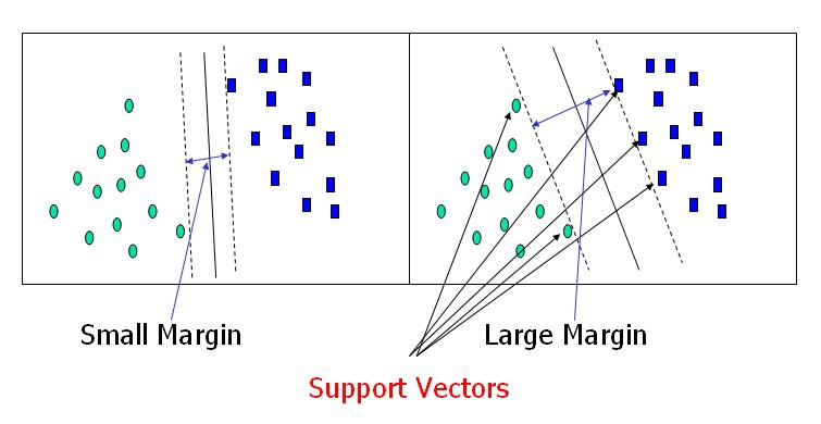
Support vectors are data points closer to the hyperplane in an N-dimensional space. A hyperplane is an N-dimensional region that provides maximum separation between two classes of data points. Support vectors influence the position and orientation of the hyperplane. Using support vectors, we maximize the margin of the classifier.
Figure: Support vectors and hyperplane
Source: https://towardsdatascience.com/support-vector-machine-introduction-to-machine-learning-algorithms-934a444fca47
See also,
rubicast
Train-Test Split
In statistics and ML, the selected data is divided into two parts – the training data and the testing data. Sometimes, it is divided into three parts, which includes validating data along with the other two. The model is fitted on the training data and then is used to make predictions on the testing data.
The training dataset contains a known output and the model is trained to learn and draw conclusions based on further inputs from any untrained/general data in the future. The testing dataset is used to test the prediction capability of the trained model.
The train/test split of a given dataset is usually around 80/20 or 70/30. This means that if 80% of the data is used for training a model, the remaining 20% is used for testing it. Similarly, if 70% data is the training data, the remaining 30% is the testing data.
True Negative
A test result that rightly indicates that a particular condition or attribute is absent can be termed as a True Negative result.
In terms of hypothesis testing, a true negative is rejecting a false null hypothesis.
In binary classification, a true negative is a situation when both the predicted outcome and the actual outcome are zero (0).
For example, in a football match, a referee declares that there is NO GOAL, and in reality too, there is a NO GOAL. In this case, the result is a true negative.
See also,
True Positive
A test result that rightly indicates that a particular condition or attribute is present can be termed as a True Positive result.
In terms of hypothesis testing, a true positive is accepting a true null hypothesis.
In binary classification, a true positive is a situation when both the predicted outcome and the actual outcome are one (1).
For example, in a football match, a referee declares that there is a GOAL and there is a GOAL in reality as well. In this case, the result is a true positive.
See also,
Word Correlation
Word correlation refers to the association or relationship between two words in a text. It determines whether and how strongly pairs of quantitative and continuous variables (in this case, words) are related to each other.
See also,
Word Frequency
Word frequency is the number of occurrences of a word in a given text.
See also,
Workbook
A workbook is a canvas to perform experiments on the data using a variety of algorithms. Workbooks are used to train datasets, which are then used in workflows.
In rubiscape, all trial and testing on the data is done in workbooks to create a list of learned datasets.
See also,
Workflow
A workflow is a canvas where a user runs the final algorithm. All tested flows, which have learned data are used here and deployed onto the production.
See also,
Workspace
A workspace is a file where you can manage multiple Datasets and Projects. Workspaces are mapped to the login, which means you may have limited access to specific workspaces as defined by your administrator.
See also,
Table of Contents

