One-Way ANOVA
Description	It compares the mean values of three or more independent groups in order to determine the statistical evidence that the associated population means are significantly different.
Why to use	To perform analysis of variance.
When to use	Equality testing between three or more population means.	When not to use	Equality testing between only two population means.
Prerequisites	Independent variables should be numerical.
Input	Any dataset that contains numerical data.	Output	Degrees of Freedom Sum of Squares Mean Sum of Squares F-Ratio
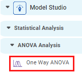
Statistical Methods used	Sum of Squares Mean Sum of Squares Shapiro Wilk Test Bartlett Test of homogeneity	Limitations	It cannot be used on any data other than numerical. It cannot be used for more than one dependent variable.

One Way ANOVA is located under Model Studio ( ) in ANOVA Analysis under Statistical Analysis, in the task pane on the left. Use the drag-and-drop method to use the algorithm in the canvas. Click the algorithm to view and select different properties for analysis. Refer to Properties of One-Way ANOVA.

One Way ANOVA is a statistical analysis method. It is used to determine if there are any statistical differences in three or more samples' mean values.

In One-Way ANOVA,

Null Hypothesis – All the samples have an equal mean.

Alternative Hypothesis – All the samples do not have equal means.

One-Way ANOVA tests the Null Hypothesis(H₀),

H₀: µ₀ = µ₁= µ₂= µ₃= … = µ_k

Where,

µ = the group mean

k = number of samples

Suppose One-Way ANOVA returns a significant result. In that case, we accept the alternative hypothesis: at least two groups have mean values that are significantly different from each other.

However, it cannot tell which groups have significantly different means.

Properties of One-Way ANOVA

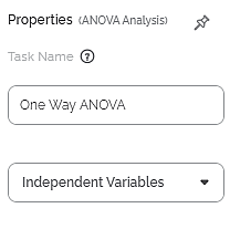
The available properties of One-Way ANOVA are as shown in the figure given below.

The table given below describes the different fields present on the properties of One-Way ANOVA.

Field	Description	Remark
Task Name	It is the name of the task selected on the workbook canvas.	You can click the text field to edit or modify the name of the task as required.
Independent Variables	It allows you to select the experimental or predictor variable(s).	Multiple data fields can be selected. Data fields with only numerical values should be selected.

Interpretation of Result of One-Way ANOVA

The table given below describes the parameters of One-Way ANOVA Test Results.

Parameter	Description	Remark
Degrees of Freedom	The number of independent values that can differ freely within the constraints imposed on them.	—
Sum of Squares	It is the sum of the square of the variations. Variation is the difference (or spread) of each value from the mean.	—
Mean Sum of Squares	It is the value obtained by diving the Sum of Squares by Degrees of Freedom.	—
F-Ratio	It is the ratio of two Mean Square values.	If the null hypothesis is true, the value of the F-ratio is closer to 1.0
p Value	It is the probability of obtaining the observed results, or more extreme, of a hypothesis test, assuming that the null hypothesis of the study question is true.	If p value < 0.05, we accept the alternative hypothesis. If p value > 0.05, we do not reject the null hypothesis.
W Stats	It tests whether a random sample comes from a normal distribution. Shapiro Wilk Test and Bartlett Test both generate this value.	If the W Stats value is small, the null hypothesis is rejected, and it can be concluded that the random sample is not normally distributed.
Shapiro Wilk Test	Null Hypothesis – The collected samples are from a normally distributed population. Alternative Hypothesis – The collected samples are from a population that is not normally distributed.	If p value < 0.05, we accept the alternative hypothesis. If p value > 0.05, we do not reject the null hypothesis.
Bartlett Test	Null Hypothesis – All the samples have the same variance. (They have homogeneity in variance.) Alternative Hypothesis – All the samples do not have the same variance.	If p value < 0.05, we accept the alternative hypothesis. If p value > 0.05, we do not reject the null hypothesis.

Example of One-Way Anova

Consider an example of a manufacturing plant that uses different packaging methods. The number of products packed per minute by five different methods - A, B, C, D, and E, is given below.

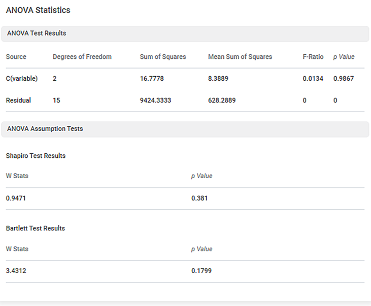
We apply One-Way ANOVA on the above data. The result is displayed in the figure given below.

In the above figure,

The p-value for ANOVA Analysis is 0.9867
The p-value for Shapiro Wilk Test is 0.381
The p-value for the Bartlett test is 0.1799

Since p-value of ANOVA (0.9867) is greater than 0.05, we conclude that the population is normally distributed, and all the samples have the same variance.

Table of Contents