Two-Way ANOVA
Description	It analyzes the effect of independent variables on the expected outcome along with their relationship to the outcome itself.
Why to use	To perform analysis of variance.
When to use	To know how two independent variables, in combination, affect a dependent variable.	When not to use	When the number of dependent variables is more than one.
Prerequisites	The dependent variable should be continuous. One independent variable should be categorical. One independent variable should be numerical. All the independent variables should be taken from a normally distributed population.
Input	Any dataset that contains numerical data.	Output	Degrees of Freedom Sum of Squares Mean Sum of Squares F-Ratio
Statistical Methods used	Shapiro Wilk Test Bartlett Test of homogeneity	Limitations	It cannot be used on any data other than numerical. It cannot be used for more than one dependent variable.

Two Way ANOVA is located under Model Studio ( ) in ANOVA Analysis under Statistical Analysis, in the task pane on the left. Use the drag-and-drop method to use the algorithm in the canvas. Click the algorithm to view and select different properties for analysis. Refer to Properties of Two Way ANOVA.

Two-Way ANOVA is a statistical analysis method. It is used to determine if there are any statistical differences in two or more samples' mean values.

In Two-Way ANOVA,

Null Hypothesis –

There is no difference in group means of the first independent variable.
There is no difference in group means of the second independent variable.

Alternative Hypothesis – All the samples do not have equal means.

Two Way ANOVA tests the Null Hypothesis (H₀),

H₀: µ₀ = µ₁= µ₂= µ₃= … = µ_k

Where,

µ = the group mean

k = number of samples

A two-way ANOVA is used to estimate how the mean of a quantitative variable changes according to the levels of two categorical variables. Use a two-way ANOVA when you want to know how two independent variables, in combination, affect a dependent variable.

Properties of Two-Way ANOVA

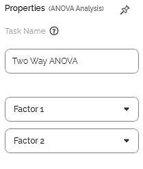
The available properties of the Two Way ANOVA are as shown in the figure given below.

The table given below describes the different fields present on the properties of Two Way ANOVA.

Field	Description	Remark
Task Name	It is the name of the task selected on the workbook canvas.	You can click the text field to edit or modify the name of the task as required.
Factor 1	It allows you to select the independent variables with numerical values.	Multiple data fields can be selected.
Factor 2	It allows you to select the categorical independent variables.	Multiple data fields can be selected.

Interpretation of Result of Two-Way ANOVA

The table given below describes the parameters of One-Way ANOVA Test Results.

Parameter	Description	Remark
Degrees of Freedom	The number of independent values that can differ freely within the constraints imposed on them.	—
Sum of Squares	It is the sum of the square of the variations. Variation is the difference (or spread) of each value from the mean.	—
Mean Sum of Squares	It is the value obtained by diving the Sum of Squares by Degrees of Freedom.	—
F-Ratio	It is the ratio of two Mean Square values.	If the null hypothesis is true, the value of the F-ratio is closer to 1.0
p Value	It is the probability of obtaining the observed results, or more extreme, of a hypothesis test, assuming that the study question's null hypothesis is true.	If the p value < 0.05, we reject the null hypothesis.
W Stats	It tests whether a random sample comes from a normal distribution. Shapiro Wilk Test and Bartlett Test both generate this value.	If the W Stats value is small, the null hypothesis is rejected, and you can conclude that the random sample is not normally distributed.
Shapiro Wilk Test	Null Hypothesis – The collected samples are from a normally distributed population. Alternative Hypothesis – The collected samples are from a population that is not normally distributed.	If p value < 0.05, we reject the null hypothesis. If p value > 0.05, we do not reject the null hypothesis.
Bartlett Test	Null Hypothesis – All the samples have the same variance. (They have homogeneity in variance.) Alternative Hypothesis – All the samples do not have the same variance.	If p value < 0.05, we reject the null hypothesis. If p value > 0.05, we do not reject the null hypothesis.

Example of Two-Way ANOVA

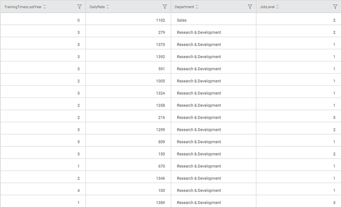
Consider an example of HR dataset. A data snippet for average yield of seeds in first three quarters over the past few years is shown in the figure below.

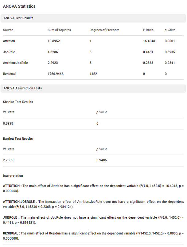
We use Two-Way ANOVA on the above data. The result is displayed in the figure given below

In the above figure,

The p-value for ANOVA Analysis is 0.0001
The p-value for Shapiro Wilk Test is 0
The p-value for the Bartlett test is 0.9486

Since the p-value of ANOVA is 0.0001 which is significant (< 0.05), implies the variable (time in years) has significant impact on the yield. The p-value of Shapiro Test is 0 which is significant (< 0.05), we conclude that the data is not normally distributed. The p-value of Bartlett test is 0.9486 which is not significant (> 0.05), we conclude that there is homogeneity of variance in the data.

Table of Contents