Ridge Regression
Description	Predict and analyze data points as output for multiple regression data that suffer from multicollinearity by controlling the magnitude of coefficients to avoid over-fitting.
Why to use	Predictive Modeling
When to use	To regularize the regression, if the Sum of Squared Residuals is too high or too low.	When not to use	On Textual data.
Prerequisites	If the data contains any missing values, use Missing Value Imputation before proceeding with Ridge Regression. If the input variable is of categorical type, use Label Encoder. The output variable must be a continuous data type. Linearity – The relationship between the dependent and independent variables is linear. Independence – The variables should be independent of each other. Normality – The variables should be normally distributed. The Dependent variable (Y) vs. Residuals plot must not follow a pattern. The errors should be normally distributed.
Input	Any continuous data	Output	The predicted value of the dependent variables.
Statistical Methods used	Fit Intercept Dimensionality Reduction	Limitations	It cannot be used on textual data.

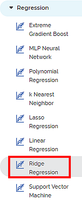
Ridge Regression is located under Machine Leaning ( ) under Regression, in the left task pane. Use the drag-and-drop method to use the algorithm in the canvas. Click the algorithm to view and select different properties for analysis.

Refer to Properties of Ridge Regression.

Regularization techniques are used to create simpler models from a dataset containing a considerably large number of features. Regularization solves the problem of over-fitting to a great extent and helps in feature selection.

Initially, L1 regularization (Lasso Regression) reduces the number of features by decreasing the coefficients of less important features to zero. After that, the L2 regularization, also called the Ridge Regression, introduces a penalty term to further reduce the magnitude of the remaining features' coefficients. The addition of penalty decreases the difference between the actual and the predicted observations.

Thus, Ridge regression solves the problem of multicollinearity in linear regression. Multicollinearity results when independent variables in a regression model are found to be correlated, and this can have a negative impact on the model fitting and interpretation of results.

Hence, when the magnitude of coefficients is pushed close to zero, the models work better on new datasets and are better optimized for prediction.

Properties of Ridge Regression

The available properties of Ridge Regression are as shown in the figure given below.

The table given below describes the different fields present on the properties of Ridge Regression.

Field		Description	Remark
Task Name		It is the name of the task selected on the workbook canvas.	You can click the text field to edit or modify the name of the task as required.
Dependent Variable		It allows you to select the dependent variable.	You can select only one variable, and it should be of numeric type.
Independent Variables		It allows you to select independent variables.	You can select more than one variable. You can select variables of any type. If categorical or textual variables are selected, you need to use Label Encoders.
Advanced	Alpha	It allows you to enter a constant that multiplies the L1 term.	The default value is 1.0.
	Fit Intercept	It allows you to select whether you want to calculate the value of constant (c) for your model.	You can select either True or False. Selecting True will calculate the value of the constant. The default value is True.
	Maximum Iteration	It allows you to enter the maximum number of iterations.	—
	Tolerance	It allows you to enter the precision of the solution.	The default value is 0.001.
	Solver	It allows you to select the method to use to compute the Ridge coefficients.	The available methods are: Auto - It selects the solver automatically based on the type of data. Auto is the default value. Svd - It uses a Singular Value Decomposition of X. Cholesky – It uses the standard scipy.linalg.solve function. Sparse_cg - It uses the conjugate gradient solver. Lsqr - It uses the dedicated regularized least-squares routine. It is the fastest. Sag – It uses Stochastic Average Gradient descent. Saga – It uses an improved, unbiased version of Stochastic Average Gradient descent.
	Random State	It allows you to enter the seed of the random number generator.	This value is used only when Selection is set to random, and the Solver method selected is Sag or Saga.
	Dimensionality Reduction	It allows you to select the method for dimensionality reduction.	The available options are – None and PCA. The default value is None.
	Add result as a variable	It allows you to select whether the result of the algorithm is to be added as a variable.	For more details, refer to Adding Result as a Variable
	Node Configuration	It allows you to select the instance of the AWS server to provide control on the execution of a task in a workbook or workflow.	For more details, refer to Worker Node Configuration.
	Hyper Parameter Optimization	It allows you to select parameters for optimization	For more details, refer to Hyper Parameter Optimization

Interpretation of Ridge Regression

Ridge Regression performs L2 regularization in order to enhance the accuracy of the prediction. It shrinks the coefficients.

The equation for Ridge Regression is, y = β₀ + β₁x + (α * (slope)²)

The larger the value of alpha, the model becomes less sensitive to variations of the independent variable.

Example of Ridge Regression

Consider a dataset of Credit Card balances of people of different gender, age, education, and so on. A snippet of input data is shown in the figure given below.

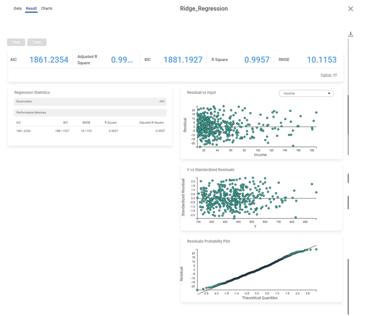
We select Limit, Balance, Income, Cards, and Age as the independent variables and Rating as the dependent variable. The result of Ridge Regression is displayed in the figure below.

The table below describes the various performance metrics on the result page.

Performance Metric	Description	Remark
RMSE (Root Mean Squared Error)	It is the square root of the averaged squared difference between the actual values and the predicted values.	It is the most commonly used metric to evaluate the accuracy of the model.
R Square	It is the statistical measure that determines the proportion of variance in the dependent variable that is explained by the independent variables.	Value is always between 0 and 1.
Adjusted R Square	It is an improvement of R Square. It adjusts for the increasing predictors and only shows improvement if there is a real improvement.	Adjusted R Square is always lower than R Square.
AIC (Akaike Information Criterion)	AIC is an estimator of errors in predicted values and signifies the quality of the model for a given dataset.	A model with the least AIC is preferred.
BIC (Bayesian Information Criterion)	BIC is a criterion for model selection amongst a finite set of models.	A model with the least BIC is preferred.

Table of Contents