Extreme Gradient Boost Classification
Description	Extreme Gradient Boost (XGBoost) is a Decision Tree-based ensemble algorithm. XGBoost uses a gradient boosting framework. It approaches the process of sequential tree building using parallelized implementation.
Why to use	Regardless of the dataset and the type of prediction task, i.e., Classification or Regression in hand XGBoost Algorithm performs best and is robust to overfitting.
When to use	To solve the prediction problems for Regression and Classification.	When not to use		Large and unstructured dataset.
Prerequisites	If the input dataset has categorical attributes, you need to use Label Encoder. It can only be used for the structured dataset.
Input	Any dataset that contains categorical, numerical, and continuous attributes.	Output	Classification Analysis characteristics - Key Performance Index, Confusion Matrix, ROC Chart, Lift Chart, and Classification Statistics.
Statistical Methods used	Accuracy Sensitivity Specificity F Score Confusion Matrix ROC Chart Lift Chart Classification Statistics	Limitations	It is efficient for only small to medium size-structured or tabular data.

Note:

There is no need to implement scaling and normalization over continuous attributes in the input dataset since the XGBoost is a non-parametric algorithm.

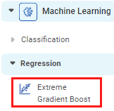
Extreme Gradient Boost is located under Machine Learning () in Classification, in the task pane on the left. Use the drag-and-drop method (or double-click on the node) to use the algorithm in the canvas. Click the algorithm to view and select different properties for analysis.

Refer to Properties of Extreme Gradient Boost.

XGBoost algorithm falls under the category of supervised learning. It can be used to solve both regression and classification problems.

XGBoost is a Decision Tree-based algorithm. A decision tree is used in classification when the predicted outcome is the class to which the data belongs. A decision tree builds a classification model in the form of a tree structure. It breaks down a dataset into smaller and smaller subsets while at the same time an associated decision tree is incrementally developed. The more the depth of the tree, the more accurate the prediction is. For more information about the Decision Tree algorithm refer to, Decision Tree.

XGBoost uses the ensemble learning method. In this method, data is divided into subsets and passed through a machine learning model to identify wrongly classified data points. Using this outcome, a new model is built to further identify the wrongly classified data points. Depending on the dataset size and desired level of accuracy, the process continues for a fixed number of iterations. It reduces the number of wrongly classified data points and thus increasing accuracy. The resultant output is obtained by aggregating outcomes of multiple machine learning models.

Note:

Rubiscape provides a separate XGBoost algorithm for Regression. For details, refer to Extreme Gradient Boost Regression (XGBoost).

Properties of Extreme Gradient Boost

The total available properties of the XGBoost classifier are as shown in Properties and Advance Properties figures given below.

The advanced properties of XGBoost classifier are as shown in the figure given below.

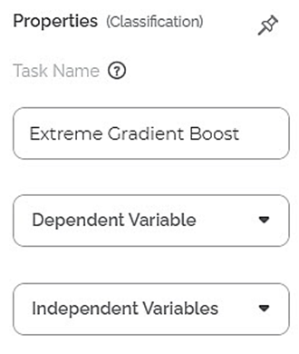
The table below describes the different fields present on the Properties pane of the XGBoost Classifier, including the basic and advanced properties.

Field		Description	Remark
Task Name		It displays the name of the selected task.	You can click the text field to edit or modify the name of the task as required.
Dependent Variable		It allows you to select the variable for which you want to perform the task.	Only one data field can be selected. Only a categorical data field can be selected.
Independent Variables		It allows you to select the experimental or predictor variable(s).	You can select more than one variable. You can select variables of any type. If categorical variables are selected, you need to use Label Encoder.
Advanced	Learning Rate	It allows you to set the weight applied to each classifier during each boosting iteration.	The higher learning rate results in an increased contribution of each classifier.
	Number of estimators	It allows you to enter the number of estimators. Estimator stands for Trees. It takes the input from the user for the number of trees to build the ensemble model.	The default value is 100. It does not have a fixed upper limit. The maximum value is selected in such a way that it will help in XGBoost’s robustness.
	Maximum Depth	It allows you to set the depth of the Decision Tree.	It is advisable to choose an optimum depth. More depth also takes more time and computation power.
	Booster Method	It allows you to select the booster to use at each iteration.	The available options are, gbtree gblinear dart gbtree and dart are optimization methods used for classification problems, whereas; the gblinear method is used for a regression problem.
	Alpha	It allows you to enter a constant that multiplies the L1 term.	The default value is 1.0.
	Lambda	It allows you to enter a constant that multiplies the L2 term.	The default value is 1.0.
	Gamma	It allows you to enter the minimum loss reduction required to make a further partition on a leaf node of the tree.	The range is 0 to ꝏ. The default value is 0.0.
	Sub Sample Rate	It allows you to enter the fraction of observations to be randomly sampled for each tree.	The range is 0 to 1. The default value is 1.0.
	Column Sample for Tree	It allows you to enter the subsample ratio of columns when constructing each tree.	The range is 0 to 1. The default value is 1.0.
	Column Sample for Level	It allows you to enter the subsample ratio of columns for each level.	The range is 0 to 1. The default value is 1.0.
	Column Sample for Node	It allows you to enter the subsample ratio of columns for each node, i.e., split.	The range is 0 to 1. The default value is 1.0.
	Random state	It allows you to enter the random state value	Only numerical values can be entered. The default value is 0.
	Dimensionality Reduction	It allows you to select the dimensionality reduction technique.	Only one data field can be selected. The available options are, None PCA The default value is None.
	Node Configuration	It allows you to select the instance of the AWS server to provide control on the execution of a task in a workbook or workflow.	For more details, refer to Worker Node Configuration.
	Hyperparameter Optimization	It allows you to select parameters for Hyperparameter Optimization.	For more details, refer to Hyperparameter Optimization.

Example of Extreme Gradient boost

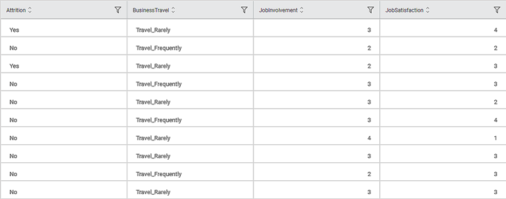
Consider an HR dataset that contains various parameters. Here, three parameters - Age, Distance from home, and Monthly Income are selected to perform the attrition analysis. The intention is to study the impact of these parameters on the attrition of employees. We analyze which factors have the most influence on the attrition of employees in an organization.

A snippet of input data is shown in the figure given below.

The selected values for properties of the XGBoost classifier are given in the table below.

Property	Value
Dependent Variable	Attrition
Independent Variables	Age, Distance from home, and Monthly Income
Learning Rate	0.3
Number of estimators	100
Maximum Depth	6
Booster Method	gbtree
Alpha	0.0
Lambda	1.0
Gamma	0.0
Sub Sample Rate	1.0
Column Sample for Tree	1.0
Column Sample for Level	1.0
Column Sample for Node	1.0
Random state	0
Dimensionality Reduction	None
Node Configuration	None
Hyperparameter Optimization	None

XGBoost Classifier gives results for Train as well as Test data.

The table given below describes the various Key Parameters for Train Data present in the result.

Field	Description	Remark
Sensitivity	It gives the ability of a test to identify the positive results correctly.	It is also called the True Positive Rate. The obtained value of sensitivity for the XGBoost Classifier is 0.998 after performing analysis.
Specificity	It gives the ratio of the correctly classified negative samples to the total number of negative samples.	It is also called inverse recall. The obtained value of specificity for the XGBoost Classifier is 0.8241 after performing analysis.
F-score	F-score is a measure of the accuracy of a test. It is the harmonic mean of the precision and the recall of the test.	It is also called the F-measure or F-score. The obtained value of the F-score for the XGBoost Classifier is 0.9814 after performing analysis.
Accuracy	Accuracy is the ratio of the total number of correct predictions made by the model to the total predictions.	The obtained value of Accuracy for the XGBoost Classifier is 0.9685 after performing analysis.
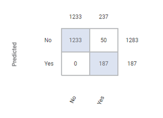
Precision	Precision is the ratio of the True positive to the sum of True positive and False Positive. It represents positive predicted values by the model	The obtained value of precision for XGBoost classifier is 0.961 after performing the analysis.

The Confusion Matrix obtained for the XGBoost Classifier is given below.

A confusion matrix, also known as an error matrix, is a summarized table used to assess the performance of a classification model. The number of correct and incorrect predictions are summarized with count values and broken down by each class.

The Table given below describes the various values present in the Confusion Matrix.

Field	Description	Remark
True Positive (TP)	It gives an outcome where the model correctly predicts the positive class.	Here, the true positive count is 187.
True Negative(TN)	It gives an outcome where the model correctly predicts the negative class.	Here, the true negative count is 1233.
False Positive (FP)	It gives an outcome where the model incorrectly predicts the positive class when it is actually negative. It is called as Type 1 error.	Here, the false positive count is 0.
False Negative(FN)	It gives an outcome where the model incorrectly predicts the negative class when it is actually positive. It is called a Type 2 error.	Here, the false negative count is 50.

Note:

The model that has minimum Type 1 and Type 2 errors is the best fit model.

The ROC and Lift charts for the XGBoost Classifier are given below.

The table given below describes the ROC Chart and the Lift Curve

Field

Description

Remark

ROC Chart

The Receiver Operating Curve (ROC) is a probability curve that helps measure the performance of a classification model at various threshold settings.

ROC curve is plotted with True Positive Rate on the Y-axis and False Positive Rate on the X-axis.
The area under the ROC curve (AUC) is a performance metric used to measure the efficiency of a machine learning model.
The value range of AUC is between 0 to 1, where 0 being the less efficient model and 1 being the best fit one.
In the above graph, the ROC curve is very close to the ideal value 1.

Lift Chart

A lift is the measure of the effectiveness of a model.
It is calculated as a ratio of the results obtained with and without the predictive model.

A lift chart contains a lift curve and a baseline.
It is expected that the curve should go as high as possible towards the top-left corner of the graph.
The greater the area between the lift curve and the baseline, the better is the model.
In the above graph, the lift curve remains above the baseline up top 80% of the records and then gradually reaches the baseline.

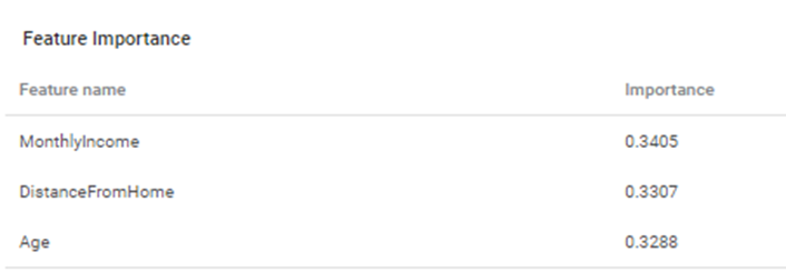
The table of classification characteristics is given below. It explains how the selected features affect the attrition for the given HR data. The importance of features is displayed in descending order. The feature that affects the attrition rate the most is displayed on top. The feature that affects the attrition the least is displayed at the bottom. Here, Monthly Income is displayed at the top as it has the most impact on attrition, and Age is displayed at the bottom as it has the least impact on attrition.

Table of contents