Decision Tree is located under Machine Learning ( ) in Classification, in the task pane on the left. Use drag-and-drop method to use the algorithm in the canvas. Click the algorithm to view and select different properties for analysis.

Refer to Properties of Decision Tree.

Decision tree algorithm falls under the category of supervised learning. It can be used to solve both regression and classification problems.

Decision tree is used in classification when the predicted outcome is the class to which the data belongs. Decision tree builds classification model in the form of a tree structure. It breaks down a dataset into smaller and smaller subsets while at the same time an associated decision tree is incrementally developed. The final result is a tree with decision nodes and leaf nodes. A decision node has two or more branches. Leaf node represents a classification or decision and internal node represent attributes of the tree.

Any Boolean function with discrete attributes can be represented using the decision tree.

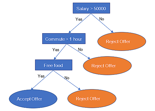
Let us take a simple example of a person considering a new job offer. A simple decision tree is shown in the below figure.

As seen in the above figure, a person’s decision to accept or reject a job offer depends on a number of conditions. At each intermediate node, a condition is verified and based on the answer (Yes/No), the decision-making process continues. All the leaf nodes denote the decision based on the attributes preceding that node.

Properties of Decision Tree

The available properties of Decision Tree are as shown in the figure given below.

The table given below describes the different fields present in the properties of Decision Tree.

Concepts in Decision Tree

When we are trying to build the Decision Tree, we start with a root node and recursively add child nodes until we fit the training data perfectly. The problem that we face is to determine which attribute in a given set of training feature vectors is most useful for discriminating between the classes to be learned.

To do this we use entropy & information gain.

Entropy

It is used to calculate homogeneity of a sample. It gives us the measure of impurity in our class. It can be roughly thought of as how much variance the data has. The lesser the entropy the better the output. The entropy typically changes when we use a node in a decision tree to partition the training instances into smaller subsets.

The lesser the entropy, the better the output is.

Information Gain

Information gain can be understood as decrease in "uncertainty" once the value of the attribute is known. Information gain is a measure of this change in entropy. Information gain tells us how important a given attribute of the feature vectors is. We can use it to decide the ordering of attributes in the nodes of a decision tree.

A feature with highest Information Gain is selected as the next split attribute.

Assume there are two classes P and N and let the set of training data S (with a total number of object s) contain p element of class P and n elements of Class N. So, entropy is calculated as,

Entropy = -(n/s) log(n/s) -(p/s) log(p/s)

Information Gain can be thought of as how much Entropy is removed or how unpredictable the dataset is.
So, Information Gain = 1 – Entropy

The lesser the value of Information Gain, the better the dataset is.

Gini

Similar to Entropy, it gives us the measure of impurity in our class. It is used to decide the next attribute to split the data on. The formula to calculate Gini Index is,

Gini = 1 -  ∑(n/s)²

A feature with a lower Gini Index is selected as the next split attribute.

Interpretation from results of Decision Tree

Sensitivity

In binary classification, sensitivity (also called a true positive rate or hit rate or recall) is the ability of a test to correctly identify the positive results. Thus, it is the ability to test positive where the actual value is also positive. 

It is quantitatively measured as the True Positive Ratio (TPR) given by

TPR = TP / (TP + FN)

Where,

TP = number of true positives

FN = number of false negatives

Specificity

In binary classification, specificity (also called inverse recall) represents the proportion of negative results that were correctly classified. It is the ratio of the correctly classified negative samples to the total number of negative samples.

It is quantitatively measured as

Specificity = TN / (TN + FP)

Where,

TN = number of True Negatives

FP = number of False Positives

F-Score

In binary classification, F-score (also called the F-measure or F₁ score) is a measure of the accuracy of a test. It is the harmonic mean of the precision and the recall of the test.

It is calculated as,

F-score = 2 (precision × recall) / (precision + recall)

Where,

precision = positive predictive value, which is the proportion of the positive values that are positive

recall = sensitivity of a test, which is the ability of the test to correctly identify positive results to get the true positive rate. 

The best F-score is 1 where the test delivers the perfect precision and recall, while the worst F-score is 0 which indicates the lowest precision and lowest recall.

Accuracy

Accuracy (of classification) of a predictive model is the ratio of the total number of correct predictions made by the model to the total predictions made. Thus,

Accuracy = (TP + TN) / (TP + TN + FP + FN)

Where,

TP, TN, FP, and FN indicate True Positives, True Negatives, False Positives, and False Negatives respectively.

Multiplying this ratio by 100 converts it into a percentage. Model classifiers have a 100% accuracy which is not possible.

Many times, classification accuracy can be misleading. Hence it is desirable to select a model with a slightly lower accuracy because it has a higher predictive power in the classification problem.

Confusion Matrix

Confusion matrix (also called the error matrix) is a summary of the results of the predictions on a classification problem. It is used to calculate the performance of a classifier on a set of testing data where the true values are already known.

A confusion matrix helps us to visualize the performance of a classification algorithm.