Inverse Cumulative Distribution Function

Inverse Cumulative Distribution Function
Description	Inverse Cumulative Distribution Function (ICDF) is the inverse of Cumulative Distribution Function (CDF). It helps to learn about the distribution of data by calculating the value associated with a specific cumulative probability in the dataset.
Why to use	To determine the value of the variable or feature associated with a specific probability.
When to use	For numerical variables having positive integer values.	When not to use	For numerical variables having values less than 0.
Prerequisites	The values of datapoints should be in the range between 0 and 1. The data should not contain any missing values.
Input	One numerical variable having values between 0 and 1.	Output	ICDF Curve Quantile values predicted by the ICDF
Statistical Methods used	Quantile function Probability	Limitations	It can be used only on numerical data.

Inverse Cumulative Distribution Function is located under Model Studio ( ) in Statistical Analysis, in the left task pane. Use the drag-and-drop method to use the algorithm in the canvas. Click the algorithm to view and select different properties for analysis.

Refer to Properties of Inverse Cumulative Distribution Function.

The Inverse Cumulative Distribution Function determines the original value of the randomly selected variable for the given probability value from the dataset.

By default, the data is sorted and then sent to the algorithm. Also, in the output Data tab, the resultant data appears in a sorted manner.

Properties of Inverse Cumulative Distribution Function

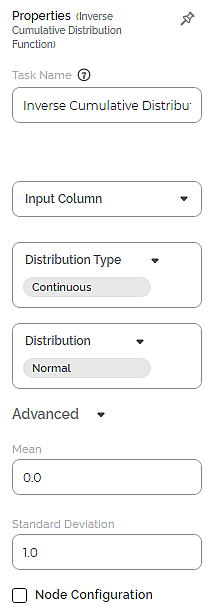
The available properties of the Inverse Cumulative Distribution Function are as shown in the figure given below.

The table below describes the different fields present on the Properties pane of the Inverse Cumulative Distribution Function.

Field		Description	Remark
Task Name		It is the name of the task selected on the workbook canvas.	You can click the text field to edit or modify the name of the task as required.
Input Column		It allows you to select the variable to be selected as the input attribute.	You can select any numerical type of variable. If the data contains missing values, you have to impute the missing values before using the Cumulative Distribution Function. To convert the values beyond the range of 0 to 1 into the required range (between 0 to 1), you can apply the normalization technique in data scaling. (Note: Scaling operation converts the values in the range of -1 to 1.)
Distribution Type		It allows you to select the type of distribution to be applied to the data.	There are two types of Distribution to select from: Continuous Discrete
Distribution		It allows you to select the sub-type of the Distribution selected above.	The sub-types present in Continuous and Discrete Distribution are given in Description of Advanced Options for Distribution Type and Distribution Pairs.
Advanced	Node Configuration	It allows you to select the instance of the AWS server to provide control on the execution of a task in a workbook or workflow.	For more details, refer to Worker Node Configuration.

In the Advanced options, algorithmic parameters for ICDF also appear according to the pair of Distribution Type and Distribution selected. These parameters change according to the Distribution Type and Distribution selected.

For example, when you select the Inverse Cumulative Distribution Function node, the option for Distribution Type is Continuous and that for Distribution is Normal. In this case, the parameters that appear in the Advanced Options are Mean and Standard Deviation.

The table given below describes these two parameters.

Table: Description of Advanced Options for Continuous Distribution Type and Normal Distribution

Field	Description	Remark
Mean	It allows you to select the mean value corresponding to the normal distribution.	It appears by default when the Distribution Type is Continuous, and Distribution is Normal. The default value for Mean is 0.0.
Standard Deviation	It allows you to select the value of standard distribution corresponding to the normal distribution.	It appears by default when the Distribution Type is Continuous, and Distribution is Normal. The default value for Standard Deviation is 1.0.

The table below gives the other parameters that appear in advanced options available for individual Distribution Types and Distribution pairs.

Table 6: Description of Advanced Options for Distribution Type and Distribution Pair for Inverse Cumulative Distribution Function

Distribution Type	Distribution	Parameter in Advanced Options	Description
Continuous	Chi-squared	Degrees of Freedom	The default value is 1. You can select the minimum and maximum values (integers) as 1 and 30, respectively.
	Standard Exponential	—	The applicable parameters are already configured.
	Exponential	Alpha (α)	You can select any real float value greater than zero.
	F-distribution	Degree of Freedom 1	The default value for both the Degrees of Freedom is 1. You can select the minimum value as zero (0). Any value above zero can be selected as the maximum value.
	F-distribution	Degree of Freedom 2
	Gamma	Alpha (α)	The default value is 1. You can select any integer value greater than zero.
	Standard Normal	—	The applicable parameters are already configured.
	Normal	Mean	The default value is 0.0. You can select any value in the range from − ∞ to ∞ (minus infinity to infinity).
	Normal	Standard Deviation	The default value is 1.0. You can select any value greater than zero.
	t	Degrees of Freedom	The default value is 1. You can select the minimum and maximum values (integers) as 1 and 30, respectively.
	Standard Uniform	—	The applicable parameters are already configured.
	Continuous Uniform	Lower Limit	The default value is 1.
	Continuous Uniform	Upper Limit	The default value is 2. Upper limit should always be greater than lower limit value. Both the upper and lower limit values lie in the range from − ∞ to ∞ (minus infinity to infinity).
	Weibull_min	Shape Parameter	The default value is 1. You can select any value greater than zero.
	Weibull_max	Shape Parameter	The default value is 1. You can select any value greater than zero.
	Beta	Alpha	The default value is 1. You can select any value greater than zero.
	Beta	Beta	The default value is 1. You can select any value greater than zero.
	cauchy	—	The applicable parameters are already configured.
	lognormal	Sigma	The default value is 1. You can select any value greater than zero.
Discrete	Binomial	Number of trials	The default value is 10. You can select the minimum value as zero (0). You can select any real value greater than zero (0) as the maximum value.
	Binomial	Probability	The default value is 0.5. You can select the minimum and maximum values (float) as 0 and 1, respectively.
	Geometric	Probability	The default value is 0.5. You can select the minimum and maximum values (float) as 0 and 1, respectively.

Example of Inverse Cumulative Distribution Function

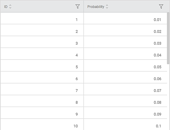
Consider a dataset of Probability values for various IDs. A snippet of input data is shown in the figure given below.

The selected values for properties of the Inverse Cumulative Distribution Function are given in the table below.

Property	Value
Input Column	Probability
Distribution type	Continuous
Distribution	Exponential
Alpha	1.0

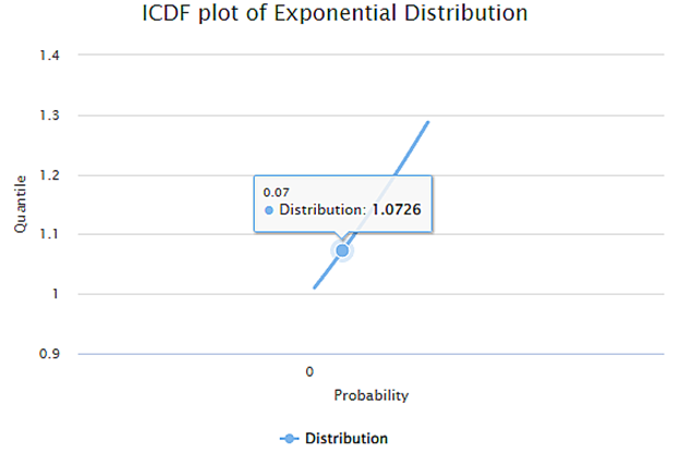
The Result page of the Inverse Cumulative Distribution Function is displayed in the figure below. The graph shows the variation in Quartile values for the probability values in the dataset.

For example, the Probability for the data point 0.7 has a Quartile value of 1.0726.

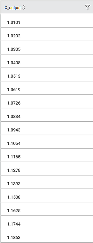
The Data page of the Inverse Cumulative Distribution Function is displayed in the figure below. It shows a snippet of the X_output values, the Quartile values, corresponding to Probability values in tabular form. By default, the values of Petal Width are sorted and arranged in an ascending order.

Table of Contents