Lag
Description	Lag, also called the sliding window method, is a backshift operator function. The window width is the number of places the data points are shifted.
Why to use	Lag is used to create a new list of data points by shifting them by an integral number of places.
When to use	To create a shifted list of variables	When not to use	When the data does not contain trend or seasonal factor
Prerequisites	The dataset should contain at least one data point.
Input	Any time-series data	Output	Dataset with values moved to successive positions
Statistical Methods Used	—	Limitations	—

Lag is located under Forecasting ( ) in Data Preparation, in the left task pane. Use the drag-and-drop method to use the algorithm in the canvas. Click the algorithm to view and select different properties for analysis.

Refer to Properties of Lag.

In Lag, no aggregation is performed on the data. The data points are shifted by an integral number of places.
The lag function is also called the sliding window method. The window width indicates the number of places the data points are shifted.
For example, a width of one (1) indicates that in the Lagged column,

the first entry is NA
subsequent entries are the same as the original column with a shift of one place. Hence in the Lagged data column, the subsequent rows are filled with the values from the previous row in the original column.

Properties of Lag

The available properties of Lag are as shown in the figures given below. Figure 2 below shows the basic configurations for Lag.

The table given below describes the different fields present on the properties of Lag.

Field		Description	Remark
Task Name		It is the name of the task selected on the workbook canvas.	You can click the text field to edit or modify the task's name as required. Space between words is not allowed in the Task Name.
Time ID Variable		It allows you to select the time variable.	The dataset should contain at least one time variable.
Target Variable		It allows you to select the variable for performing the Lag.	The variable selected should be discrete.
Group By		It allows you to select the function for grouping identical data.	Identical values of a column variable in different rows are grouped. Usually, the variable selected is categorical. Selecting Group By is optional
Advanced	Interval	It allows you to select the interval you want to calculate the Lag.	The available options are: Day Week Month Quarter Year By default, the interval is set to Month.
	Start Time	It allows you to select the time beginning which the data is sliced.	By default, the value is None.
	End Time	It allows you to select the time ending in which the data is sliced.	By default, the value is None.
	Lag	It allows you to select the number by which the data points are shifted	You can select any integral value. By default, the value is 1.
	Node Configuration	It allows you to select the instance of the AWS server to provide control on the execution of a task in a workbook or workflow.	For more details, refer to Worker Node Configuration.

Example of Lag

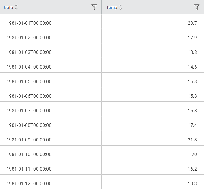
Consider a Temperature dataset with 10 records. It contains columns for Date and corresponding daily temperature. A snippet of the input data is shown in the figure below.

We apply Lag to the input data. The selected values for Lag are given below.

Property	Value
Time ID Variable	Date
Target Variable	Temp
Group By	—
Interval	Day
Start Time	None
End Time	None
Lag	2

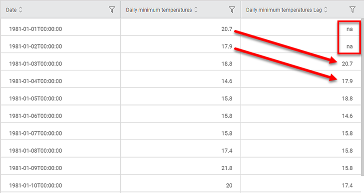
On the Data pane, you see that

the first two values in the Temp Lag column are 'na.'
Values in the Temp column are shifted two places in the Temp Lag column

Table of Contents