Train Test Split in Forecasting
Description	The data is split randomly into train data and test data. Ideally, the split is in the ratio of 70:30 or 80:20 for Train and test.
Why to use	To evaluate the accuracy of the model with an unknown dataset.
When to use	The dataset contains a large number of rows.	When not to use	Limited data is available.
Prerequisites	In Forecasting, the data should NOT be shuffled because it contains seasonality. Hence the date stamp and its sequence are very crucial. (For this reason, shuffling is disabled in Forecasting. That is, it is taken as False for Train Test Split.)
Input	Any dataset that contains any form of data – Textual, Categorical, Date, Numerical data.	Output	Dataset split into two parts – Train data and Test data.
Statistical Methods used	--	Limitations	If the data is limited, then there is a possibility of high bias.

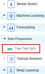
Train Test Split is located under Forecasting ( ) in Data Preparation, in the left task pane. Use the drag-and-drop method to use the algorithm in the canvas. Click the algorithm to view and select different properties for analysis.

Refer to Properties of Train- Test Split.

The train-test split is a technique to evaluate the accuracy of a model. It is used to make predictions on a large dataset. It is appropriate where a good quick estimate of the model performance is required.

In this technique, the input dataset is divided into two datasets, Train, and Test. The train dataset is used to fit the model by getting the model trained on the input dataset. The expected output of the data is known. The test dataset is used to make predictions on unknown data. It evaluates the performance of the model on new data.

The data in each of the Train and test sets should ideally represent the problem. There should be enough records to cover all common and uncommon cases of the problem or situation. If the dataset size is not optimum, it may overfit or underfit the model.

Properties of Train-Test Split

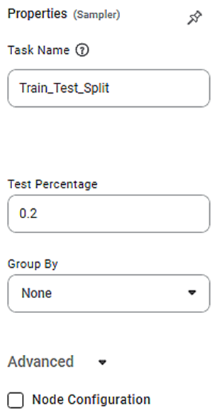
The available properties of Train Test Split are as shown in the figure below.

The table below describes the different fields present on the properties of Train-Test Split.

Field		Description	Remark
Task Name		It is the name of the task selected on the workbook canvas.	You can click the text field to edit or modify the name of the task as required.
Test Percentage		It is the percentage to divide input data into test data. The remaining percentage is train data.	The default value is 0.2. It indicates that the dataset is split into 20% test data and the remaining 80% as train data. You can select any value as required.
Group by		It allows you group the values by a column	Only one data field can be selected Only categorical data fields are available
Advanced	Node Configuration	It allows you to select the instance of the AWS server to provide control on the execution of a task in a workbook or workflow.	For more details, refer to Worker Node Configuration.

Interpretation of Train Test Split

The data is split into the train dataset and test dataset.

The split percentage is selected considering the points mentioned below.

The train set represents the dataset sufficiently
The test set represents the dataset sufficiently
The computational cost of evaluating the model
The computational cost of training the model

The common split percentage is:

Train: 80%, Test: 20%
Train: 70%, Test: 30%

Example of Train-Test Split

Consider an Superstore dataset with 63 records. It contains more than 10 columns. A snippet of the input data is shown in the figure given below.

We apply Train Test Split on the input data. The input dataset is split into train records and test records while maintaining the data sequence, based on the Test Percentage parameter given in the properties.

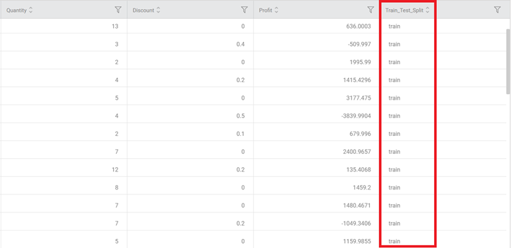
The segmentation of records into Train and test is displayed in the data column Train Test Split, as shown in the figure below.

If you scroll down the data, you notice that the train and test records are segregated to maintain the seasonality of the data.

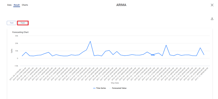
Further, we apply the time-series forecasting algorithm ARIMA (Auto-Regressive Integrated Moving Average) on the split data.

The result for Train data is displayed in the figure given below. The graph shows the variation in the sales with Ship date.

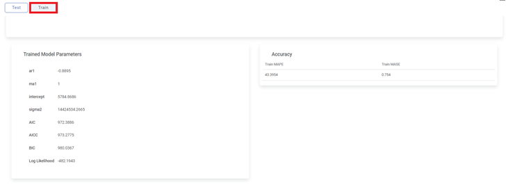
The Result page also displays the Trained Model Parameters for the ARIMA algorithm, and its Accuracy, on the same page, below the graph.

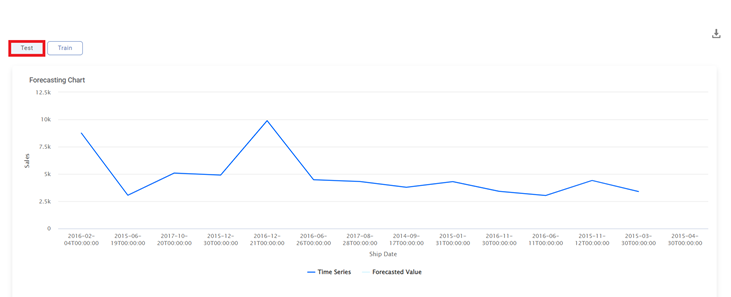
Similarly, the resulting graph for the Test data for ARIMA is displayed in the figure given below.

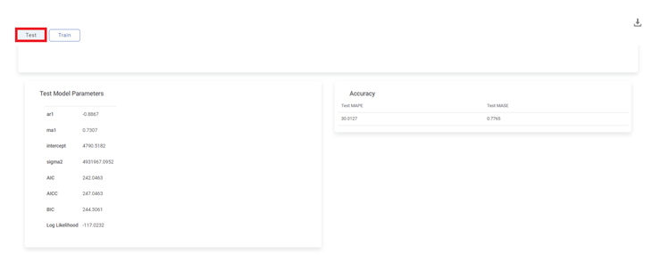
Also, the Result page displays the Trained Model Parameters for the ARIMA algorithm and its Accuracy corresponding to Test Data, on the same page, below the graph.

Similarly, you can use Train Test split to test the performance of other Forecasting algorithms.

Table of contents