Factor Analysis
Description	Factor Analysis is also known as exploratory Factor Analysis for data reduction. It is a technique of examining interdependent variables without distinguishing between dependent and independent variables. Factor Analysis extracts maximum common variance from all the variables in the data and puts them into a common score. It groups variables and reduces data. It helps researchers investigate various concepts that are otherwise difficult to measure directly. Factor Analysis identifies the underlying factors in given data. These underlying factors explain the correlation between the set of variables in the given data. It is mostly used as a prelude to multivariate analysis
Why to use	For reduction and summarization of data. To remove irrelevant data. To identify the exact number of factors that are required to explain the common themes among a given set of variables To determine the extent to which each variable in the dataset is related to the common factor
When to use	As a data preparation method before using unsupervised machine learning models When you want to identify a small set of non-correlated variables to replace the original set of correlated variables to be used in subsequent multivariate analysis. When you want to develop a hypothesis about the relationship between variables When you want to spot trends and themes in your dataset	When not to use	When the data is already known with an identified set of dependent and independent variables. When the variables are limited in number and sufficient to describe the trends in data.
Prerequisites	The dataset should be sufficiently large with a large number of variables. Outliers should not be present in the data. The variables in the data should not possess a perfect multicollinearity There is a linear relationship between variables Only relevant variables should be included in the analysis, and there should be a true correlation between the variables and factors
Input	Variables that are non-classified as independent and dependent	Output	Factors that group the variables based on their correlation
Statistical Methods used	Factor loading scores KMO test accuracy score Uniqueness extraction Communality extraction Correlation Chart Factor Plot Scree Plot Bartlett Test of Sphericity Chi-square value Degrees of Freedom Sigma Eigenvalue PCA Maximum Likelihood	Limitations	Factor Analysis cannot be used if there is a defined correlation between variables. After a factor is identified, naming the factor can be a difficult task Factor Analysis reveals an apparent structure in the data even if the variables are extremely random. It may lead to confusion about whether the factor explains the data. It is difficult to decide the number of factors to be retained. The interpretation of the significance of factors is subjective, and the reasoning given by different people can be different.

Factor Analysis is located under Model Studio ( ) in Data Preparation, in the left task pane. Use the drag-and-drop method to use the algorithm in the canvas. Click the algorithm to view and select different properties for analysis.

Refer to Properties of Factor Analysis.

To illustrate the significance of Factor Analysis, let's consider an example.
Consider three groups of customers choosing three different detergent powder brands. Each group has its reasons for selecting a particular brand. These reasons are compiled in the form of three different sets of data. Each dataset contains variables/features related to information about the group's choices. Then, in this example, Factor Analysis brings out those factors responsible for the choice of a brand.
There are two hypotheses in Factor Analysis.

Null Hypothesis: There is no significant correlation between the variables.
Alternative Hypothesis: There is a significant correlation between the variables.

It analyzes variables that have an interdependence. This interdependence is examined and established only after the Factor Analysis is completed because we do not classify variables as dependent and independent. All variables before Factor Analysis are treated as independent.
Using Factor Analysis, we reduce the number of variables, and in this process, group the similar variables and remove the irrelevant ones.

Steps in Factor Analysis:

Define the problem statement as to why you want to perform Factor Analysis
Construct the Correlation Matrix
Determine the Pearson Correlation between variables and identify which variables are correlated.
Decide the method to be taken up for Factor Analysis
1. Rotation for Varimax
2. Maximum Likelihood
Determine the number of relevant factors for the study. For example, you have a set of seven variables, and you want to reduce them to three. It is an individual decision based on the dataset and analytical requirements. (This is mostly determined using the trial and error methodology)
Rotate the factors and interpret the results.

Properties of Factor Analysis

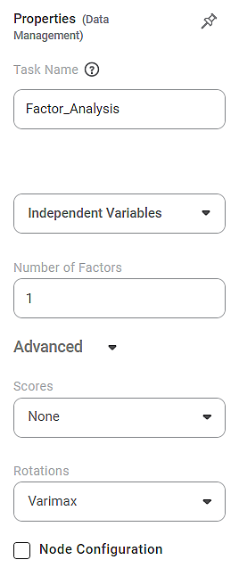
The available properties of the Factor Analysis are shown in the figure below.

The table below describes the different fields present on the Properties pane of the Chi-Square Goodness of Fit Test.

Field		Description	Remark
Task Name		It is the name of the task selected on the workbook canvas.	You can click the text field to edit or modify the task's name as required. To read more about the algorithm/functionality, hover over the Help Icon ( ) next to the Task Name heading.
Independent Variable		It allows you to select the unknown variables to determine the factors.	You can select any numerical data type of variable as an independent variable. These variables are reduced to common attributes called factors used for regression or modeling purposes. In Factor Analysis, all the variables are considered independent.
Number of Factors		It allows you to select the number of factors you want to reduce the number of variables.	By default, the number of factors is one (1). The number of factors is always an integer value. Normally, you should select a number less than the number of independent variables in the dataset. It is because the aim of Factor Analysis is data reduction. The number of factors is one less than the number of variables.
Advanced	Scores	It allows you to select the factor score for Factor Analysis.	It is also known as the component score. The following methods are available for calculating the factor score. None Regression (default) Bartlett Selection of None value means that no score is selected The Bartlett score is a test statistic (sigma value) used to explain the null hypothesis; that is, the variables are not correlated in the dataset. Generally, if the Bartlett score is less than 0.05, Factor Analysis is recommended.
	Rotations	It allows you to select the factor rotation method.	The factor rotation method decides how the axes are rotated so that factors undergo multiple rotations, and we obtain the best possible combination of variables for a given factor. By default, the method selected is Varimax. You can select from the following methods. None Varimax Promax Selection of None value means that the factor rotation method is not selected. Varimax is an orthogonal rotation method. It constrains the factors to be non-correlated. It minimizes the number of variables with high factor loading on each factor. It simplifies the factor interpretation. Promax is an oblique rotation method. It allows the correlation of factors. Promax is useful for large datasets since it can be calculated quickly. Varimax is a more common and recommended method of factor rotation.
	Node Configuration	It allows you to select the instance of the AWS server to provide control over the execution of a task in a workbook or workflow.	For more details, refer to Worker Node Configuration.

Results of Factor Analysis

The following table elaborates on the findings obtained from Factor Analysis.

Result

Significance

Loadings

Factor Loadings show how much a factor can explain a variable.
The range of factor loadings is from -1 to 1.
The values of factor loadings close to -1 or 1 show that the factor has a huge influence on the variable.
If the factor loading is close to zero, this influence is weak.
Some factors may have a simultaneous high influence on multiple variables.

KMO Test (Kaiser-Meyer-Olkin Test)

The KMO test measures the suitability of data for Factor Analysis.
It measures whether each variable has an adequate sample in the model and the complete model.
The test yields a statistic called the KMO statistic.
It measures the proportion of variance that the variables have with each other, which might have a common variance.
The value of the KMO statistic lies between 0 and 1.
The following table gives the interpretation of various KMO values.

KMO Value	Interpretation
Close to zero	Widespread correlation among the variables
Less than 0.6	Inadequate Sampling Action is needed to resolve the sampling issue. Any KMO statistic below 0.5 is unacceptable.
Between 0.6 & 1	Adequate Sampling Any KMO statistic above 0.9 is considered excellent

Note: Practically, a KMO accuracy value above 0.5 is also considered acceptable for the validity of the test. Below 0.5, the value indicates that more data collection is essential since the sample is inadequate.|

Uniqueness

Uniqueness gives the value of variance unique to a variable.
It is not shared with any other variable in the dataset.
Uniqueness = 1 – Communality,
- Where communality is that variance that it shares with the other variables.
- For example, a communality of 0.75 means a uniqueness of 0.25 in the variable. Thus, the variable has 75% variance from other variables and only 25% uniqueness.
A greater uniqueness value indicates that the variable is less relevant for factor analysis.

Communalities

Communality is the common variance found in any variable.
It is an important measure to determine the value of a variable in Factor Analysis (or Principal Component Analysis).
Communality tells us what proportion of the variable's variance results from the correlation between the variable and the individual factors.
In Factor Analysis, communality is denoted by h².
The communality of a variable lies between 0 and 1.
If the communality of variance is 0, the variable is unique. It cannot be explained by any other variable at all.
If the communality is 1, the variable does not have any unique variance and can be completely explained using other variables.

Practically, the values of communality extraction for a variable should be greater than 0.5. You can remove the variable and re-run the Factor Analysis in such a case.

Note: However, values of 0.3 and above are also considered depending on the dataset.

Correlation Chart

A correlation matrix shows the correlation values between the variables.
It gives the Pearson correlation coefficient values to measure the linear correlation between the two variables
The correlation values vary from -1 (strong negative correlation) to 1 (strong positive correlation).
A correlation value of zero (0) indicates that the relation between the two variables is orthogonal. That is, they are not correlated at all.

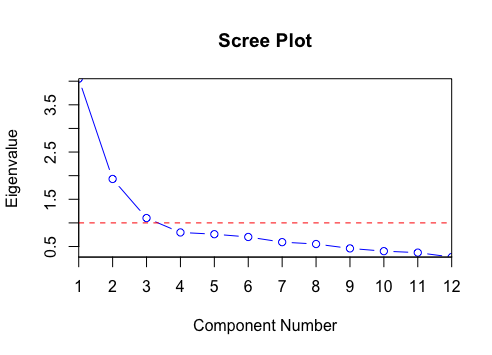
Scree Plot

A scree plot is a line graph that essentially plots and displays the eigenvalues in a multivariate analysis.
The eigenvalues are
- factors that need to be retained in the exploratory factor analysis, or
- principal components that need to be retained in the principal component analysis.
The eigenvalues are plotted on the Y-axis on a scree plot, while the number of factors is plotted on the X-axis.
A scree plot displays these eigenvalues in a downward curve from largest to the smallest.
- The first factor or component usually explains a major part of the variability.
- The subsequent few components explain the variability moderately, while the components after that explain only a minuscule fraction of the variability.
The scree plot results from the scree test, a method to determine the most significant factors or components.
- The 'elbow point' (where the eigenvalues seem to be leveling off) is determined from this test.
- All eigenvalues to the left of this elbow are considered significant and are retained, while the values to the right are non-significant and are discarded.

Bartlett Test of Sphericity

Bartlett's test of sphericity is a test of comparison between the observed correlation matrix and the identity matrix.
Bartlett's test checks
the redundancy between variables
and whether we can reduce the redundant variables so that the data can be summarized with only a few factors.
For Bartlett's test,
Null Hypothesis: The variables are orthogonal. That is, they are not correlated.
Alternate Hypothesis: The variables are not orthogonal. That is, they are correlated.
Thus, Bartlett's test ensures that the correlation matrix diverges prominently from the identity matrix. It helps us in selecting the data reduction technique.
This test yields a p-value which is then compared with the chosen significant level represented by a significance value (usually, 0.01. 0.05, or 0.1 are chosen as significance values.)
If the p-value is less than the significant level, the data set contains redundant variables and is suitable for the data reduction technique.

Example of Factor Analysis

Consider a dataset containing time required in seconds and minutes by international athletes in a track event. Variables X1 to X7 are the seven events, each containing the times required by athletes from various countries. The variables are so labeled to hide the identity of the type of event.
A snippet of the input data is shown in the figure given below.

For applying Factor Analysis, the following properties are selected.

Independent Variables	X1, X2, X3, X4, X5, X6, and X7
Number of Factors	3
Scores	None
Rotation	Varimax

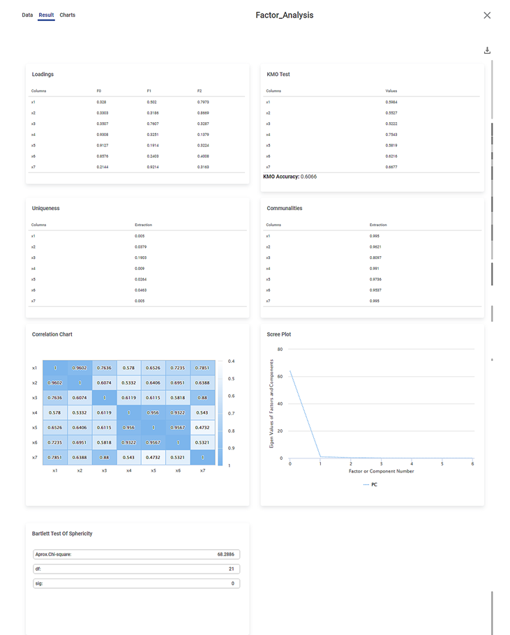
The image below shows the Results page of the Factor Analysis.

We first look at the Bartlett Test of Sphericity results on the Results page, followed by the KMO Test. The statistics and results obtained in these two tests are crucial to deciding whether the Factor Analysis is required.
Bartlett's Test of Sphericity tells you whether you can go ahead with the Factor Analysis for data reduction. KMO test tells you whether the Factor Analysis is appropriate and accurate.

Bartlett Test of Sphericity:

The Approximate value of Chi-Square = 60.2886
Degrees of Freedom (df) = 21
Sigma (sig) = 0

Inference:

Since the sigma value (0) is less than the p-Value (assumed as 0.05), the dataset is suitable for data reduction, in our case, Factor Analysis.
It also indicates a substantial amount of correlation within the data.

KMO Test:

You can see the individual KMO values for each variable.
- It is 0.5984 for X1, 0.5527 for X2, and so on.
The overall KMO accuracy is 0.6066 (greater than 0.6).

Inference:

Since the individual KMO scores for each variable are greater than 0.6, the individual data points are adequate for Sampling.
Since the overall KMO score is greater than 0.6, the overall Sampling is adequate.

After the results from these two tests are analyzed, you can study other results. Among the remaining, you first analyze the communality extraction values for various variables.

Communalities:

You can see the communality extraction score for each variable.
- It is 0.995 for X1. 0.9621 for X2, and so on.
- It is maximum for X4 (0.991) and minimum for X3 (0.8097).

Inference:

The closer the communality is to one (1), the better is the variable explained by the factors.
- Hence, X4 is the most explained variable, while X5 is comparatively the least explained variable.
The closer the communality extraction values for variables, the better the chances of the variables belonging to a group (or community) and having a communal variance.
For example, X1, X2, and X4 have high chances of belonging to a group.

Loadings:

You can see the variance values of a variable as determined by each factor.
- For example, the variance of variable X1 is better explained by factor F2 (0.7973) compared to F0 (0.328).
- The variance of variable X4 is better explained by factor F0 (0.9308) compared to F1 (0.3251).
The factor loading scores indicate which variables fall into which factor category to be combined.
- X1 and X2 will fall into the F2 group
- X3 and X7 will fall into the F1 group
- X4,X5, and X6 will fall into the F0 group

Notes:

In unsupervised machine learning, the variables X1, X2, and so on are unknown.
After Factor Analysis, the variables are grouped into factors, and then the factors are suitably named.
For example, you want to stitch shirts for students in a class. You take each student's Height and Shoulder Width measurements (variables) and then classify them into sizes Small, Medium, and Large (factors) as required.|

Uniqueness:

You can see the uniqueness extraction values for each variable.
It is 0.005 for X1, 0.0379 for X2, and so on.
It is maximum for X3 (0.1903) and minimum for X1 (0.005).
Uniqueness is calculated as '1- Communality'. It means that more communal is a variable, less is its uniqueness.
Thus, X3 is the most unique, while X1 is the least unique value.

Correlation Plot:

It gives the values of Pearson correlation for all the variables.
A value of Pearson correlation closer to one (1) indicates a strong correlation between two variables, while a value close to zero (0) indicates a weak correlation.
For example, variable X1 is more strongly correlated to X2, while X4 is more strongly correlated to X7.

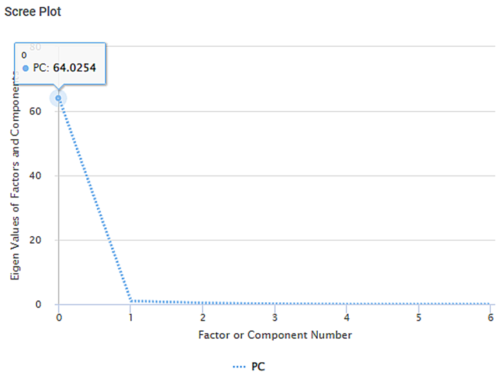
Scree Plot:

It plots the eigenvalues of factors against the factor number
The PC (Principal Component) value for
the zeroth factor is 64.0254,
for the first factor is 1.013, and so on
You see an elbow near the first factor. Only the factors to the left of the elbow are retained, and those to the right of the elbow are discarded.
Hence, only the zeroth factor is retained, and all the remaining factors are discarded.

+

Table of contents