Density Based Clustering
Description	It classifies the given set of data by building clusters based on the idea that a cluster in the data space is a continuous region of high point density, separated from other clusters by continuous regions of low density.
Why to use	It works well to separate data areas with a high density of observations from data areas that are not very dense with observation. DBSCAN can sort data into clusters of arbitrary shapes as well.
When to use	When the number of clusters is not known. When there is too much noise in data. To separate data points of high density from data points of low density.	When not to use	When the number of clusters is known.
Prerequisites	Input data should be of text type and should not contain special characters and numbers.
Input	Textual Data	Output	Data divided into clusters.
Statistical Methods used	Ball tree Kd tree Brute	Limitations	It does not work well in the case of high-dimensional data or with clusters of varying densities.

Density Based Clustering is located under Textual Analysis ( ) in Clustering, in the left task pane. Use the drag-and-drop method to use the algorithm in the canvas. Click the algorithm to view and select different properties for analysis.

Refer to Properties of Density Based Clustering.

Density-based clustering is an unsupervised learning method. It identifies distinctive clusters in data to be the regions of high point density, clearly separated from other clusters by a region of low point density. These separating regions of low point density are considered as noise or outliers.
In density-based clustering, core samples of high point density are identified, and clusters are developed from them. This method is suitable for data that contains data of comparable density. Also, clusters found in density-based clustering can be of any shape as opposed to the k-means method, where clusters are assumed to be convex-shaped.

Properties of Density Based Clustering

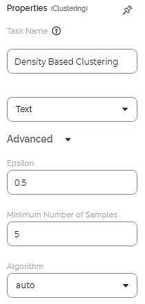
The available properties of Density Based Clustering are as shown in the figure given below.

The table given below describes the different fields present on the properties of Density Based Clustering.

Field		Description	Remark
Task Name		It is the name of the task selected on the workbook canvas.	You can click the text field to edit or modify the name of the task as required.
Text		It allows you to select Independent variables.	You can select more than one variable. You can select any type of variable.
Advanced	Epsilon	It allows you to enter the maximum distance between two data points for them to be considered in the neighborhood of each other.	The default value is 0.5
	Minimum Number of Samples	It allows you to enter the minimum number of samples to be considered while assigning clusters.	The default value is 10.
	Algorithm	It allows you to select the algorithm to be used for searching the nearest neighbor while assigning clusters.	The available options are – Auto – It determines the algorithm among Ball_tree, Kd_tree, and Brute that is best suited for the input dataset. Ball_tree – It divides the data points into two clusters, and each cluster is contained by either a circle or a sphere. Kd_tree – It divides the data points into two sets at each node. Brute – It uses the brute-force method to compute distances between all pairs of data points.

Example of Density Based Clustering

Consider a dataset of Musical Instruments review. A snippet of input data is shown in the figure given below.

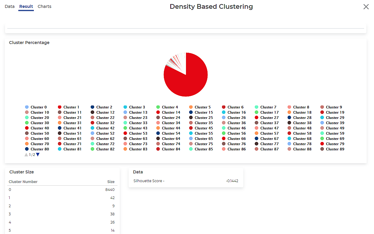
After using the Density Based Clustering, the following results are displayed.

As seen in the above figure, each cluster's size is mentioned along with the Silhouette Score.

Table of Contents